


The surveys outlined in Section 3 have transformed our pictures and physical understanding of the nature of high-redshift star-forming galaxies. The development of resolved kinematic measurements at z > 1 to complement photometric ones has allowed deeper evolutionary connections to be made between galaxies in the early Universe and locally. Whilst the story is by no means complete, some clear physical pictures, which one might call useful 'working models' to prove further (or refute), of the nature and structure of these galaxies have emerged which I will attempt to summarise here. I will defer outstanding observational and physical questions to the final section.
An important early question was whether disc galaxies existed at all at high-redshift (Baugh et al. 1996, Weil et al. 1998, Mao et al. 1998). The existence of a disc presupposes some degree of gas settling, the fact that most high-redshift star-forming galaxies at high redshift showed much higher star-formation rates than those locally (Bell et al. 2005, Juneau et al. 2005) and also exhibited lumpy, somewhat irregular morphologies (Glazebrook et al. 1995b, Driver et al. 1995, Abraham et al. 1996b, Abraham et al. 1996a) led some to hypothesise that perhaps they were all mergers: after all the highest star-formation rate objects locally are merger-driven ULIRGS and early versions of the Cold Dark Matter model predicted high merger rates at high-redshift from hierarchical growth (Baugh et al. 1996, Weil et al. 1998). Of course not every galaxy could be seen in a merger phase, but if imaging surveys were mostly sensitive to high star-formation rate galaxies this could be interpreted as a selection effect. Is it possible that the cosmic star-formation history is merger driven (Tissera 2000)?
An alternative viewpoint is that a typical massive galaxy's star-formation history could be dominated by continuous star-formation, with a higher value than today as the galaxy would be more gas rich in the past. In this scenario, we would expect the gas and young stars to have settled in to a rotating disc. In the more modern ΛCDM model, the different expansion history tends to produce a lower merger rate than flat Ωm = 1 CDM models and the late time evolution of large galaxies is less rapid (Kauffmann et al. 1999e). Further to this new analytic arguments and hydrodynamical simulations have suggested mechanisms where galaxies sitting in the centre of haloes can continuously accrete new gas at significant rates of via 'cold cosmological flows' (Dekel et al. 2009b, Dekel et al. 2009a). Observationally, the revelation of a tight star-formation rate - stellar mass 'main sequence' whose locus evolves smoothly with redshift is also more in accord with a continuous accretion process dominating the star-formation; stochastic merger-driven bursts would introduce too much scatter in this main sequence (Noeske et al. 2007, Daddi et al. 2007, Rodighiero et al. 2011). The merger rate has been derived from close pair counts in high-redshift data (see Section 5.4, at z > 1 it is about 0.1-0.2 per Gyr (for typically mass-ratios > 1/4)). If all star-forming galaxies were undergoing mergers (with a duty cycle of 1-2 Gyr) then the rate would have to be 3-4× higher. Direct comparisons can be made of observed galaxy growth vs those predicted by mergers, e.g. Bundy et al. (2007) who compared the rate of production of observed 'new spheroids' in each redshift bin with merger rates from simulations and Conselice et al. (2013) who compared empirical merger growth from pair-counts vs the 'in-situ' growth calculated from their measured star-formation rates. These analyses favour in-situ type processes for galaxy star-formation and quenching.
Kinematic studies have been motivated by these results and as we have seen in Section 3 a large fraction (~ 30% or larger) of galaxies seen at high-redshift are clearly rotating discs, i.e. while the broad-band with HST appears photometrically irregular the objects appear kinematically regular (Bournaud et al. 2008, van Starkenburg et al. 2008, Puech 2010, Jones et al. 2010, Förster Schreiber et al. 2011, Genzel et al. 2011), a key point. Generally, the rest-frame UV and Hα from AO IFS trace each other (Law et al. 2009) whereas the stellar mass is smoother (but still clumpy) (Förster Schreiber et al. 2011, Wuyts et al. 2012). The fraction of discs seems to increase towards higher stellar masses (Förster Schreiber et al. 2009, Law et al. 2009). The typical rotation velocities are 100-300 km s-1 so very similar to local galaxies (Cresci et al. 2009, Gnerucci et al. 2011b, Vergani et al. 2012). The big surprise has been the high values of the velocity dispersion found in galaxy discs. First observed by Förster Schreiber et al. (2006) and Genzel et al. (2006) typical dispersion values (in all surveys) range from 50-100 km s-1. It is helpful to frame this as v / σ, the ratio of circular rotation velocity to dispersion. For the larger discs (stellar masses > 5 × 10¹⁰ M⊙) v / σ typically ranges from 1-10 at z ~ 2 (van Starkenburg et al. 2008, Law et al. 2009, Förster Schreiber et al. 2009, Gnerucci et al. 2011b, Genzel et al. 2011). There are also a number of objects that appear not to be dominated by rotation with v / σ ≲ 1; this class has been called 'dispersion-dominated objects' (Law et al. 2009, Kassin et al. 2012). These values compare with a value of ~ 10-20 for the Milky Way and other similar modern day spiral discs (Epinat et al. 2010, Bershady et al. 2010). If these measured values of the dispersions correspond to the dynamics of the underlying mass distribution these high-redshift discs are 'dynamically hot'.
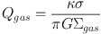
A simplified physical picture of such objects was first described by Noguchi (1998, 1999) and is nicely summarised by Genzel et al. (2011). (For a more detailed theoretical treatment see Dekel et al. 2009a). The arguments goes as follows. The classical Toomre (1964) parameter Q for stability of a gas disc is:
 |
(14) |
where Σ is the mass density and κ is the epicyclic frequency. κ = a v / R where a is a dimensionless factor 1 < a < 2 depending on the rotational structure of the disc, v is the circular velocity, and R is some measure of the radius (for an exponential disc the scalelength). The Q parameter can be understood by considering a gas parcel large enough to collapse under self-gravity despite it's velocity dispersion, i.e. larger than the 'Jeans length' LJ ≃ σ2 / G Σ. However, as gas parcels rotate around with the disc in their reference frame they also experience an outward centrifugal acceleration ≃ LJ κ2; if this is larger than the gravitational acceleration G Σ then the disc is stable. Local spiral discs tend to have Q ~ 2 (van der Kruit & Freeman 1986).
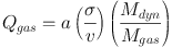
Following Genzel, if we express the total dynamical mass as Mdyn = v2 R / G and the total gas mass as π R2 Σgas then equation 14 can be rewritten as
 |
(15) |
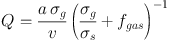
Since we expect rapidly star-forming discs to be unstable and have Q ~ 1 we arrive at the important result:
 |
(16) |
i.e. that it is a high gas fraction that gives rise to these dynamically hot discs. For a mixture of gas and young stars in a disc, if they share the same velocity, velocity dispersion, and spatial distribution, then equations 14 and 16 are still valid with the substitutions Qgas → Qyoung, Σgas→ Σyoung, fgas→ fyoung. 21 Since young stars will form from the gas on timescales less than an orbital time, it is natural to expect them to share the same distributions, and this is observed in the Milky Way (Luna et al. 2006).
For the range of 2 < v / σ < 4 typically observed derived gas fractions are 25-50%, which accords with observations of molecular gas fractions at high-redshift (Tacconi et al. 2010, Tacconi et al. 2013, Daddi et al. 2010c, Carilli & Walter 2013) A corollary of course is that since the gas/young stars fraction is not close to 100% (except possibly in the case of the 'dispersion dominated galaxies' discussed in Section 5.2), there must be another component; the fractions defined in equation 15 are relative to the total dynamical mass (and noting that the observational data from molecular gas surveys are usually relative to the total gas + stellar mass which includes young stars). For multiple components in a disc the the approximation Qeff-1 = Qgas-1 + Qstars-1 (Wang & Silk 1994) is often used (Puech et al. 2008, Genzel et al. 2011) though there are more sophisticated combinations (e.g. Rafikov 2001, Romeo & Falstad 2013). If I assume the dynamical mass is dominated by an older stellar disc (i.e fgas < 1) then I can show (using the Wang & Silk approximation and similar working to equation 15) that:
 |
(17) |
Setting Q ~ 1 and a ~ 1 I then I get:
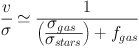 |
(18) |
which shows that the stellar dispersion needs to be several times higher than that of the gas to maintain the observed v / σ > 1 values. Alternatively, a dark matter or stellar spheroid could serve and we would expect theoretically baryon fractions of ~ 0.6 within the disc radius (Dekel et al. 2009a). In my view, it seems from the argument in Equation 18 that high-redshift discs will evolve in to local intermediate mass ellipticals or S0 galaxies (i.e. Fast Rotators), not local thick discs, as the implied stellar dispersions and masses are the right scale (100-150 km s-1, ~ 1011 M⊙). This would also follow from using the clustering properties of these high-redshift star-forming galaxies to trace descendants (e.g. Adelberger et al. 2005, Hayashi et al. 2007). Local Slow Rotators are more massive and could not form by fading of these discs, single major mergers may not be enough and these objects likely require multiple hierarchical mergers to achieve their kinematic state (Burkert et al. 2008).
Genzel et al. (2011) made maps of the Q parameter in the SINS sample and found regions of Qgas < 1 corresponded to star-formation peaks providing some support for the idea that they are clumps generated by instability (see Figure 11). However, it is critical to make the caveat that they calculated Σgas as ∝ ΣSFR0.73, i.e. using a Kennicutt-Schmidt type law, as Σgas appears in the denominator, this naturally gives low derived values of Q where the star-formation peaks. A critical test would be to repeat this using high-spatial resolution direct gas measurements.
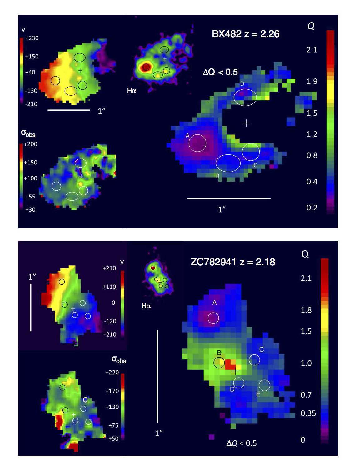 |
Figure 11. Two clumpy z ~ 2 discs from the larger sample of Genzel et al. (2011) showing velocity, dispersion, Hα and Q maps. Data is AO at resolution 0.2 arcsec. The circles denote the positions of clumps, note how these 'disappear' in to the velocity maps showing they are embedded in discs and occur in regions of Q < 1. See also Wisnioski et al. (2012) for a similar finding (but also caveat in text here). Credit: from Figures 4 & 5 of Genzel et al. (2011), reproduced by permission of the AAS. |
The other important physical parameter that arises from this picture of the Jeans length and consequent Jeans mass which sets the scale of collapsing gas clouds. The form of the Jeans length LJ ≃ σ2 / (GΣ) is the same as that for the vertical scale height of a thin disc in gravitational equilibrium h = 2π σ2 / (GΣ), thus we naturally expect the Jeans length to be similar to the disc thickness (this is also seen in simulations Bournaud et al. 2010). Putting in some numbers for high-redshift discs (σ = 70 km s-1, Mgas = 5 × 10¹⁰ M⊙, R = 3 kpc), we obtain LJ ≃ 1 kpc. The associated Jeans mass ≃ Σ LJ2 is ~ 109 M⊙. Once the clump collapses one would expect from general virial arguments that it becomes and object of virial size, a factor of two less than the Jeans length and dispersion equal to the disc dispersion (Dekel et al. 2009a). These scales and masses match those of the giant clumps of star-formation commonly observed in high-redshift galaxies supporting this model. It is the large mass scale, which can be thought of as a cut-off mass of the HII region luminosity function (Livermore et al. 2012), and fundamentally arising from a high-gas fraction, that drives the clumpy appearance to the eye as a ~ 1011 M⊙ galaxy disc can only contain a handful of such clumps. For comparison, if we consider the Milky Way with σgas = 5 km s-1 and Mgas = 3 × 10⁹ M⊙ (Combes 1991), we derive a Jeans length of ≃ 100 pc and mass of ~ 106 M⊙ which correspond nicely to the scale height of the gas disc and the maximum mass of giant molecular clouds and regions. The scale height of 1 kpc in z ~ 2 discs is similar to the scale height of the thick disc of the Milky Way (≃ 1.4 kpc, Gilmore & Reid 1983). Thick discs today tend to be old, red, and low surface brightness, however they may contain as much mass again as the bright thin disc (Comerón et al. 2011). An interesting suggestion is that these high-redshift discs could evolve in to modern thick discs if star-formation shuts down and gas is exhausted (Genzel et al. 2006). There velocity dispersions are also in accord with evolving in to lenticular galaxies today; or mergers could transform them in to massive ellipiticals.
The implication of all this is what we are observing at high-redshift are thick star-forming discs rich in molecular gas with very large star-formation complexes as I illustrated in Figure 2. Other support for this model comes from:
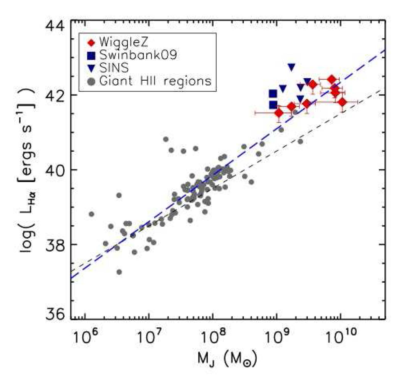 |
Figure 12. Scaling of Hα luminosity (proxy for star-formation rate) with inferred clump Jeans mass MJ = π2 r σ2 / 6G from local HII regions up to the most luminous z > 1 clumps. The correlation is quite tight and the slope close to unity (black dashed line). The blue dashed line is the best fit slope MJ1.24 Credit: reproduced from Figure 5 of Wisnioski et al. (2012). |
With typical star-formation rates of up to 50-100 M⊙ yr-1 such high-redshift galaxies would exhaust their observed gas supply in 0.5-1 Gyr. The preferred physical scenario has so far been that such galaxies are continuously supplied by cosmological 'cold flows' (Dekel et al. 2009b, Dekel et al. 2009a, Ceverino et al. 2010), with the term 'cold' denoting ~ 104 K gas that has not been shocked and virialised on entering the galaxy halo and which can flow efficiently down to the centre of a young galaxy. A 1011 M⊙ stellar mass galaxy could be smoothly assembled from star-formation in only 1-2 Gyr, a time scale comparable to the age of the Universe at z ~ 2. This is an attractive picture and also explains the tight star-formation rate-mass main sequence but some health warnings are warranted. As recently discussed by Nelson et al. (2013) who compare hydrodynamical simulations using different kinds of codes (specifically the AREPO moving mesh code and the GADGET-3 smoothed particle code), the distinction between 'cold' and 'hot' modes may be an over-simplification and can be dependent on definition and code type. Further, the delivery of large amounts of cold gas directly in to the centres of z ~ 2 galaxies may well be a numerical artefact of GADGET-3. Nevertheless, smooth accretion still dominates at z ~ 2 (compared to minor mergers) as the dominant mode of growth of large galaxies with accretion rates of up to ~ 10 M⊙ yr-1 in large haloes.
The key physical detail needed to complete this picture is the energy source powering the observed velocity dispersion. The velocity dispersions are in the supersonic regime (i.e. > 12 km s-1) and thus most likely arise from turbulent motions. However, turbulence will decay strongly on a disc crossing time 1 kpc / 70 km s-1 which is only ~ 15 Myr. At z ~ 2, the Hubble time is 3 Gyr which is much greater than the crossing time and also of orbital timescales. Since a large fraction of discs appear clumpy to maintain Q ~ 1 some sort of self-regulation is required. If σ drops then Q drops and the disc fragmentation increases, thus feedback associated with this fragmentation operating on the same timescale is a good mechanism to self-regulate (Dekel et al.2009a). In local galaxies, turbulence in the ISM is believed to be powered by star-formation feedback most likely by SNe feedback (Dib et al. 2006), though stellar winds and radiation pressure from OB stars also contribute (see review by Mac Low & Klessen 2004). At high-redshift, this has also been suggested (Lehnert et al. 2009, Le Tiran et al. 2011) which seems plausible given the connection between high dispersions and high star-formation rates; however, the absolute energetic coupling is difficult to calculate or simulate. Lehnert et al. found a correlation between spatially resolved star-formation rate surface density and velocity dispersion in the same spaxels suggesting this mechanism; however Genzel et al. (2011) found a very poor correlation in much better resolved AO data. Green et al. (2010) argued for a global correlation between integrated star-formation rates and mean dispersion. The relations between these findings is not yet clear. Other suggested mechanisms for generating high dispersions and thick discs are (i) clump-clump gravitational interaction (Dekel et al. 2009a, Ceverino et al. 2010), (ii) accretion of cold flows (Elmegreen & Burkert 2010, Aumer et al. 2010), (iii) disc instabilities and Jeans collapse (Immeli et al. 2004, Bournaud et al. 2010, Ceverino et al. 2010, Aumer et al. 2010), and (iv) streams of minor mergers (Bournaud et al. 2009). No dominant energetic picture has emerged; rather a consistent theme of these papers are that it is quite likely that there is more than one cause of high dispersion. For example, high turbulence may initially be set by the initial gas accretion of the protogalaxy, then sustained by clump formation/interaction and/or star-formation feedback. More observables to discriminate scenarios are desirable, for example the dependence of dispersion on star-formation rates (Green et al. 2010, Green et al. 2013, Genzel et al. 2011) or galaxy inclination (Aumer et al. 2010).
Another way forward in my view to further study of the energy sources powering turbulence may lie in the spatial structure that is apparent in dispersion maps, which in my view is seen consistently in all surveys (but needs AO to resolve). The dispersion varies often by factors of two across the disc. Notable examples are easy to find in the literature, for example simply inspect the dispersion maps in Figures 4, 11 and 13 of this review. The dispersion shows distinct spatial correlations which do not seem to arise simply from random noise. For comparison, the models in Figure 4 shows the dispersion should be constant (apart from a central beam-smeared peak), however the two galaxies resolved by AO have a striking asymmetry of high-dispersion regions. This point is not commented on in any of the papers. Is it real or is it a numerical artefact of the line fitting process used to create these maps? If it is an artefact, why do some galaxies show such asymmetric dispersion (e.g. ZC782941 and D3a-15504 in Figure 4) despite the velocity map being very symmetrical? If it is real, I note that it is really interesting that the dispersion seems to be higher nearer to the location of clumps but the dispersion peaks do not correspond to the star-formation peaks. This is part of the reason why the Q-maps of Genzel et al. and Wisnioski et al. show minima on the clumps (the other is the increased star-formation density). It may also explain why there seem to be divergent findings between local and global dispersion star-formation rate correlations as mentioned above. This all in my view may point to non-uniform sources of energy powering dispersion associated with nearby clumps. Since the turbulent decay time is much less than an orbital time we would naturally expect this not to be ell mixed. Demonstrating this effect is real and quantifying its spatial relation to other galactic structures would make for interesting future work.
Finally, let me end on a word of caution. Much of the work on clump properties has assumed that the dust extinction is constant across an individual galaxy. If extinction is patchy (e.g. Genzel et al. 2013) then this could cause considerable scatter in clump properties (and even in clump identification). This is a particular problem for the rest-frame UV, Hα is less affected but it is still a concern. Future resolved Balmer decrement studies combined with CO work (we expect dust to trace gas) would greatly improve our understanding of this issue.
5.2. Dispersion-dominated Galaxies
Another surprise at high-redshift was the high fraction (30-100% depending on sample definition) of galaxies which are very compact, are dominated by a single large star-forming clump, have large line widths in integrated spectra but show very little evidence for systematic rotation. This was first noticed by Erb et al. (2006a) in a sample of z > 2 Lyman Break galaxies (i.e. UV-selected) and later by Law et al. (2007, 2009) in AO follow-up of a sub-sample (see Figure 13). Objects with v/σ<1 have been labeled as 'Dispersion-Dominated Galaxies' though there is no evidence that this forms a distinct class, all surveys have shown a continuous sequence of v / σ (e.g. Figure 14). This is usually measured with circular velocity and the isotropic resolved dispersion (e.g. as measured by disc fitting or data values beam-smearing corrected in some fashion) but an important caution is that the resulting values may still depend substantially on spatial resolution due to beam-smearing (Newman et al. 2013).
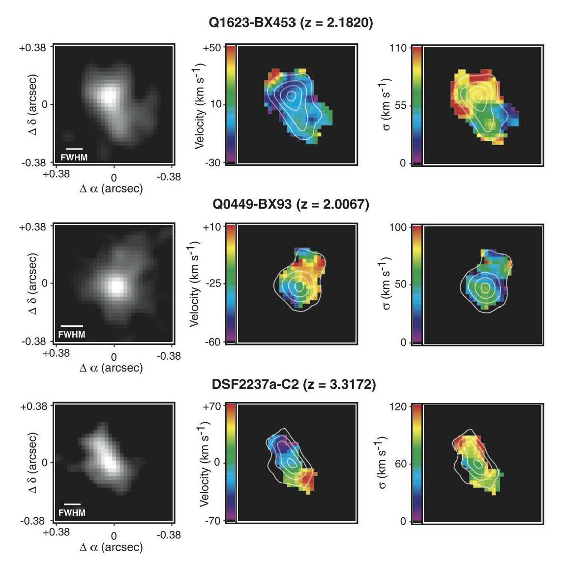 |
Figure 13. Sample UV-selected dispersion-dominated galaxies from Law et al. (2007) observed with OSIRIS AO. The columns are Hα intensity, velocity and dispersion, in all cases v≲ σ. Credit: from Figure 1 of Law et al. (2007), reproduced by permission of the AAS. |
However, the label is still useful in the sense that it is a population of galaxies that does not exist (at least in any abundance) in the local Universe but which seems to rise rapidly in number density with redshift (Kassin et al. 2012). These particular defining physical characteristics are roughly a stellar mass of 1-5 × 10¹⁰ M⊙, effective half light radii < 1-2 kpc, high star-formation rates and velocity dispersions of 50-100 km s-1 (Law et al. 2007, Law et al. 2009, Epinat et al. 2012, Newman et al. 2013). It is important to distinguish this population from that of compact red galaxies (sometimes called 'red nuggets') also seen at z ~ 2 (e.g. Daddi et al. 2005, van Dokkum et al. 2008, Cimatti et al. 2008, Damjanov et al. 2009), these have similar effective radii but have stellar masses up to a factor of ten higher (> 1011 M⊙) and are quiescent. A popular observational and theoretical scenario is that they evolve in size via minor mergers on their outskirts to become large elliptical galaxies today (Bezanson et al. 2009, Naab et al. 2009, Newman et al. 2010, Hopkins et al. 2010). Their ancestors at high-redshift (2 < z < 3) may be 'blue nuggets' (Barro et al. 2013) of similar high mass; this population has yet to be probed in detail kinematically and its relation to the dispersion-dominated galaxies at lower redshifts and lower masses is an open question. Some of the dispersion-dominated samples do contain a few high stellar mass objects (e.g. Wisnioski et al. 2011 has two with M > 1011 M⊙ with very large dispersions); though of course the stellar mass signal may be coming from a different part of the galaxy to that visible to the kinematics.
The dispersion-dominated galaxies in general form a large proportion of UV-selected samples but the fraction appears to decline with higher stellar mass (Law et al. 2009, Newman et al. 2013) as shown in Figure 14; thus, they are less common in K-selected samples. So what are dispersion-dominated galaxies physically? A simple interpretation might be that they are exactly as the observations suggest: high-star formation rate galaxies with negligible rotation and pressure supported. These would be star-forming analogs of modern day large elliptical galaxies (which also have v / σ < 1 in their stellar kinematics (Cappellari et al. 2007) but are a factor of ten more massive); perhaps they could have formed from the collapse of a single gas cloud of low angular momentum? This is also suggestive of the classical 'monolithic collapse' picture of galaxy formation of Eggen et al. (1962); however, it is important to note that monolithic collapse-type processes still have important roles in modern hierarchical models in building initial seeds for galaxy growth (Naab et al. 2007). Maybe they could simply fade to make low mass ellipticals today? One problem is we observe these galaxies to be highly star-forming, so we would suppose they are gas rich, and gas (unlike stars) dissipates very quickly. One would expect turbulent energy dissipation and settling of gas in to a cold disc to occur on a crossing time of 1 kpc / 70 km s-1 which is only ~ 15 Myr unless the turbulent energy is continuously refreshed. More generally, one would expect gas to settle in to a disc on a dynamical time which is the same. Compared to the Hubble time at this redshift, this is short, so it is unlikely that we would observe galaxies during such a brief phase.
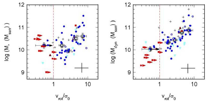 |
Figure 14. Dispersion-dominated galaxies (v / σ < 1) tend to have smaller stellar and dynamical masses but the scatter is large. (They also have smaller half-light radii not shown here). The samples are AO: red points (Law et al. 2009), blue points (SINS AO), cyan points (Swinbank et al. 2012b, 2012a), non-AO: black crosses (Lemoine-Busserolle & Lamareille 2010, Epinat et al. 2012). Grey filled circles denote median values in bins. Stellar masses are corrected to the Chabrier (2003) IMF. Credit: from Figure 7 of Newman et al. (2013), reproduced by permission of the AAS. |
There are other more natural possibilities for such objects. Since the objects are known to be small, one might hypothesise that they are simply very small disc galaxies and that some of the 'dispersion' is in fact unresolved rotation. Another possibility is that they might be 'clump cluster' disc galaxies but with only a single visible disc clump, perhaps due to their low mass. In such a scenario, the stellar mass would not all come from the clump which simply dominates the UV/Hα morphology (I note that many of the larger SINS galaxies in fact show one dominant clump sitting in an extended disc). A final possibility is that they might be newly formed bulges, at the centre of clumpy discs, after clump coalescence. In some scenarios, clumps survive long enough to migrate to the centre and merge via secular processes (Noguchi 1999, Förster Schreiber et al. 2006, Elmegreen et al. 2008). The stellar masses are in the right ball park for local bulges (Graham 2013); however, the dynamical timescale argument for star-formation still applies and it seems unlikely to find such a high fraction.
(Newman et al. 2013) present observations of 35 UV-selected z ~ 2 galaxies observed with AO as well as sources from the literature. They conclude that the 'compact disc' hypothesis is the most plausible based on extrapolations of v / σ which they find is strongly correlated with size. The stellar mass correlation is not so tight; and there are in fact some quite massive galaxies with v / σ < 1. The classification does depend on resolution in the sense that they find that if a source was classified as dispersion-dominated in natural seeing, it was quite likely to be reclassified as rotating by AO data. However, even at AO resolution there remains a substantial population of dispersion-dominated systems. The origin of the dispersion dominance is interpreted as arising partly from beam smearing in compact discs; but also as a genuine physical effect in the sense that their extrapolation of the velocity-size relation suggests that v < 50 km s-1 half-light (Hα) radii are < 1.5 kpc whilst the dispersion remains 'constant' (~ 50-70 km s-1) for galaxies of all sizes. (I note there is some evidence for dispersion increasing in the smallest galaxies, e.g. Fig. 6 in Newman et al. and Fig. 6 in Epinat et al. (2012), though this may of course also be due to beam-smearing). In such a scenario, the Jeans length is comparable to the size of the galaxy disc both radially and vertically and the entire object is one large star-forming clump as long as the observed level of turbulence can be sustained.
The scenario where there is a single clump is offset and embedded in a larger disc could be directly tested by searching for the extended galaxy. For example, HST imaging may show diffuse disc emission or even a red bulge not coincident in centre with the clump. Morphological examples do in fact exist; this is the class of galaxies known as 'tadpole galaxies' (van den Bergh et al. 1996, Elmegreen et al. 2012, Elmegreen & Elmegreen 2010). If diffuse emission spectra can be stacked then one can test for differences in the velocity centroid as a function of surface brightness. A specific morphological comparison of galaxies labeled 'dispersion dominated' with more general samples would be valuable.
5.3. Evolution of the scaling relations?
The evolution of the Tully-Fisher relationship reflects the build-up of galaxy discs. In the framework of hierarchical clustering, Mo et al. (1998) derived the following simple theoretical expression for the evolution in the disc mass Md and circular velocity Vc in isothermal dark matter haloes;
 |
(19) |
where md is the fraction of the total halo mass corresponding to the disc (typically ~ 0.05) and H(z) is the cosmological Hubble expansion rate. An assumption is that the disc vs halo mass fraction and angular momentum fraction are the same. The two pertinent features of this result are (i) that if md ≃ const., then one naturally expects a M∝ V3 stellar mass Tully-Fisher relationship and (ii) that at higher redshifts, galaxy discs could have a lower mass at fixed Vc due to the increasing H(z) factor.
So should there be an evolution in the zeropoint? One also expects the mass in the disc to be smaller at high-redshift as star-formation builds it up, so smaller md. We should also consider the effects of more realistic dark matter halo profiles (Navarro et al. 1997] and interactions between baryons and dark matter, in particular angular momentum transfer which can give rise to disc expansion or contraction (Dutton & van den Bosch 2009). A more sophisticated treatment can arise by using semi-analytic models to estimate disc rotation curves self-consistently (Somerville et al. 2008, Dutton et al. 2011a, Tonini et al. 2011, Benson 2012) or by running full hydrodynamical simulations with star-formation and feedback to follow disc galaxy evolution (Portinari & Sommer-Larsen 2007, Sales et al. 2010). Commonly it is found that the predicted evolution is along the stellar mass Tully-Fisher relationship (Dutton et al. 2011a, Benson 2012) so that the actual zero-point evolution is weak.
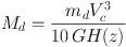
Despite the surveys outlined in Section 3, observationally, the situation is not clear. Even at low redshift, there is considerable disagreement between surveys as illustrated in Figure 15. First, there is the matter of what fraction of star-forming galaxies at different redshifts can be usefully classified as discs and placed on a Tully-Fisher relationship. Is it in the range 30-50% at 0.5 < z < 3 (Yang et al. 2008, Epinat et al. 2012, Förster Schreiber et al. 2009) or much closer to 100% (e.g. Miller et al. 2012 for z < 1.7) if one obtains deeper data? This fraction may be increased by using the S0.5 parameter which combines velocity and dispersion instead of Vc; some authors have found that this allows all galaxies, including ones with anomalous kinematics, to be brought on to a tighter Tully-Fisher relationship reducing scatter by large amounts (Kassin et al. 2007, Weiner et al. 2006a, Puech et al. 2010). However, there is debate over this true anomalous fraction and whether a tight Tully-Fisher relationship for all star-forming galaxies can be produced conventionally (Miller et al. 2011, Miller et al. 2012). Another issue is the choice of velocity parameter, for example V2.2 may be more robust and produce less scatter than Vc (Dutton et al. 2011a, Miller et al. 2012).
 |
Figure 15. A comparison of Tully-Fisher relationship findings at z < 1 for the surveys mentioned in the main text. A much larger scatter in the M-V relation is found in the sample of Kassin et al. (2012) and Puech et al. (2008) than in that of Miller et al. (2011) predominantly in objects with more disturbed morphologies. This scatter is considerably reduced in Kassin et al.'s use of the M-S0.5 relation and is then brought on to the local Faber-Jackson relation (Gallazzi et al. 2006). The disagreements are likely due to some combination of sample selection, data quality and definition of kinematic quantities but the exact combination is not yet determined. See Sections 3.8 and 5.3 for further discussion of this. Credit: kindly provided by Susan Kassin (2013). |
Neither is it yet clear whether the Tully-Fisher relationship zeropoint is observationally found to change with redshift. The range of findings is shown in Figure 16 taken from Miller et al. (2012). There certainly appears to be a lack of consistency between surveys even at moderate redshifts (~ 0.5). Some of this may be due to the methodological differences in deriving circular velocities (and perhaps stellar masses) discussed in Section 4.2. It may also be related to different choices of local relation to normalise evolution as discussed in Section 3.3. The local relations used have different slopes between them, this then will or will not cause an offset depending on the mass range probed. There is also no consistent local relation derived in a methodology which is consistent with that of high-redshift galaxies and that has been tested via simulation against redshift effects.
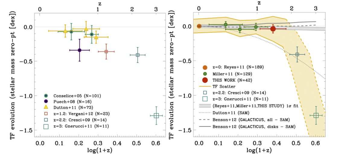 |
Figure 16. Evolution of the Tully-Fisher relationship zeropoint with redshift from Miller et al (2012). Points show zeropoint and error bars show RMS scatter around the linear relations. The left panel shows mostly previous IFS results showing considerable disagreement. The right panel shows the results from Miller et al's very deep multi-slit work claiming no evolution in the zeropoint and very small scatter to z ~ 2. Some galaxy models and empirical fits are also shown (see Miller et al. for details). There is a clear inconsistency between with the (shallower) IFS results for 0.2 < z < 2 where the redshift ranges overlap. Fast evolution at z > 2 could be possible, however deeper surveys are needed to also verify the z > 2 IFS results. The local relation is that of Reyes et al. (2011) which is based on that of Pizagno et al. (2007). Credit: from Figure 7 of Miller et al. (2012), reproduced by permission of the AAS. |
Finally, it is interesting to note that some authors have tried to compute baryonic masses for high-redshift galaxies by adding to the stellar masses an estimate of gas mass using the observed star-formation rate surface density and the Kennicutt-Schmidt relationship. There is some evidence that this works in the sense that there is usually better agreement between dynamical masses and baryonic masses than with stelar masses (Puech et al. 2010, Vergani et al. 2012, Gnerucci et al. 2011b, Miller et al. 2011). In the local Universe, the 'Baryonic Tully-Fisher relationship' is found to give a better linear relation, compared to stellar masses, down to low masses where galaxies become much more gas rich (McGaugh et al. 2000, McGaugh 2005). This has been investigated at high-redshifts; Puech et al. (2010) found no evolution in the offset of the baryonic relation at z ~ 0.6 where the stellar relation showed evolution and interpreted this as a conversion of gas in to stars from a fixed well over cosmic time. (Alternatively, one might suppose galaxies accrete gas and could move along the relation.) Similar lack of zero point evolution was found at z > 1 by Vergani et al. (2012). Given the range of results for the stellar mass zeropoint evolution (Figure 16) and the uncertainty introduced by estimating gas masses from star-formation I would argue it is premature to over-interpret the baryonic Tully-Fisher relationship evolution. The local relation uses direct HI masses; it may be another decade before HI is available in normal galaxies at z ≳ 1, but it would be interesting in the near future to consider this with estimates of molecular gas masses from CO data.
The other kinematic scaling relation is the velocity-size one. Bouché et al. (2007) found that local spirals and z ~ 2 star-forming SINS galaxies overlap substantially in this plane and there is little evidence for evolution with the exception of sub-mm galaxies which were very compact. Puech et al. (2007) found similar results at z ~ 0.6. In both cases, the scatter was considerable and not as tight as the mass-velocity relation, a result that mirrors the local Universe. Puech et al. interpreted extra scatter as arising from their disturbed kinematic classes and it is also true that the SINS sizes were for all objects, not just well-modelled discs. MASSIV finds only ≃ -0.1 dex in size-mass and size-velocity relation (i.e. smaller discs at z ≃ 1.2 compared today). Dutton et al. (2011b) note that the lack of evolution in size-velocity relations may be inconsistent with the sign of the observed Tully-Fisher relationship evolution (including those derived within the same survey such as SINS). They also compare with data from DEEP2 and size-mass relations from photometric surveys and argue there is a consistent picture of early discs being smaller, as theoretically expected, and discrepancies can be attributed to (i) different methods and conversions of size measurements, (ii) selection biases in IFS surveys, and (iii) possible differences in sizes between the young stellar populations probed by ionised gas compared to stellar mass.
One key question that IFS surveys set out to address was the prevalence of mergers at high-redshift. Certainly one might have supposed they were common given the irregular structures of high-redshift galaxies (e.g. Baugh et al. 1996) and an IFS is the instrument of choice for objects with unknown a priori kinematic axes. Merger rates can be investigated by looking at galaxy image irregularities (Conselice et al. 2003, Conselice et al. 2008, Bluck et al. 2012) but as we have seen there are numerous examples of clumpy galaxies which are morphologically irregular but kinematically regular.
Before the advent of IFS surveys the primary method of estimating the merger rate at high-redshift was via pair counts, starting with (Zepf & Koo 1989, Carlberg et al. 1994, Le Fèvre et al. 2000, Lin et al. 2004), and many papers since. By trying to estimate the fraction of galaxies that were 'interacting pairs' fint (e.g. close on the sky, using redshift and tidal feature information if available) and then adding a merger timescale Tmerge (usually calibrated via simulations) one can estimate a merger rate R:
 |
(20) |
(e.g. Bridge et al. 2010). This gives units of number of mergers per galaxy per Gyr (and can be further broken down by galaxy mass, merger mass ratio, etc.). Generally the merger rate is parameterised as evolving as (1 + z)m where recent estimates are 1 < m < 3 (Bundy et al. 2009, Kartaltepe et al. 2007, Bridge et al. 2010, Lotz et al. 2011, Xu et al. 2012). The timescale Tmerg is set by dynamical friction and is around 1 Gyr (Lotz et al. 2008, Kitzbichler & White 2008, Lotz et al. 2011); noting that not all pairs identified in surveys will eventually merge and this effect is often incorporated implicitly in to the calibration (the non-merging fraction may be around 30-50% for typical observational selections; Kitzbichler & White 2008). The star-formation rate in close pairs may even be enhanced as far as 150 kpc (Patton et al. 2013) which at this distance are not likely future mergers; but such effects do make clear the point that one should be careful of selection effects in pair catalogues especially in the rest-frame optical.
In determining the galaxy merger rare from kinematics, one arrives at a similar equation:
 |
(21) |
(e.g. Puech et al. 2012, López-Sanjuan et al. 2013) where fmerge is the fraction of galaxies identified as mergers from kinematics, and T′merge is the timescale. Note this is a different timescale from equation 20 as we are now considering closer galaxies and a more advanced merger stage. However, R should be the same (for an equivalent sample) as galaxies would be conserved at all phases of the merging process (Conselice et al. 2009). One expects both timescales to be of order 1 Gyr (Puech et al. 2012) but both can vary by factors of 2-3 (Lotz et al. 2008). Chou et al. (2012) found that only ~ 20% of close pairs at z < 1 were kinematically associated, that the merging timescale was rather short (< 0.5 Gyr), and that merging was dominated by blue-blue pairs (i.e. opposed to red on red 'dry mergers').
One approach to measuring merger rates more precisely is to take a close pair catalog and confirm the kinematic association spectroscopically using slit spectroscopy (Chou et al. 2012). An interesting hybrid approach was used by López-Sanjuan et al. (2013), where they took advantage of the fact that their IFS maps were wider field than typical to count close kinematic pairs (within ~ 20 kpc and 500 km s-1) as well as advanced ongoing mergers for star-forming galaxies with 1010-10.5 M⊙. Good agreement was found by López-Sanjuan et al. between their kinematic and other's photometric surveys at 1 < z < 1.5. Their 'major merger fraction' (meaning 1:4 at least ratios) was ~ 20% over this redshift interval translating to a merger rate of ~ 0.1 Gyr-1 (this is equivalent for a typical T ′merg ≃ 2 Gyr which is what simulations typically indicate for pairs within 20 kpc (Kitzbichler & White 2008)). They found this to be consistent with lower redshift photometric studies with an overall evolution of (1 + z)4 in the rate. Extrapolation of their power-laws would predict close to a 100% merger fraction at z = 2.5 (and a rate of ~ 0.7 Gyr-1), which seems inconsistent with the results of the SINS (Förster Schreiber et al. 2009) and AMAZE-LSD surveys (Gnerucci et al. 2011b) which both observe kinematic fractions of closer to ~ 30%. One possibility is these surveys may be missing close pairs which have not yet progressed to the kinematic stage, however the MASSIV data by itself suggests a constant rate at z > 1 so perhaps the power-law evolution could be flattening off at z > 1. A direct comparison of merger fractions and rates from purely photometric pairs would be valuable at 2 < z < 3. (Bluck et al. 2009) looked at pairs (mass ratio 1:4) within 30 kpc of > 1011 M⊙ galaxies at 1.7 < z < 3, the inferred merger rate is ~ 1 Gyr-1 (their Fig. 3) which seems consistent with the higher MASSIV extrapolation; however, the mass range is different and would include a substantial fraction of quiescent non-star-forming galaxies than does MASSIV and SINS. Slit surveys of z ~ 3 LBGs seem to find a surprisingly high fraction of spectroscopic pairs (i.e. double lined) which could also imply a higher merger rate (Cooke et al. 2010). Such a high merger/interaction rate at z > 2 typically does not match modern ΛCDM model predictions, (Bertone & Conselice 2009), (though see Cooke et al. for a contrary view).
Another possible tension is at z ~ 0.6. The IMAGES survey find a high-fraction of galaxies with anomalous IFS kinematics (Neichel et al. 2008, Yang et al. 2008, Hammer et al. 2009) which is interpreted as a high merger fraction, 33% involved in major mergers (Puech et al. 2012). The close pair studies mentioned above suggest the merger fraction is closer to 4% at z ~ 0.6 (e.g. see Figure 24 of López-Sanjuan et al. 2013) and if the timescales are similar then these should be comparable and clearly they are not. Puech et al. argued that a fraction of their objects were in what they called a 'post-fusion' phase, these should be compared to close pairs at an earlier epoch (z ~ 1.1) which lessens the tension due to the fast evolution in pairs with redshift.
However, the fact remains that if 33% of star-forming galaxies are deeply kinematically disturbed at only z ~ 0.6 and one must ask the question how is this compatible with the fact that the majority of star-forming large galaxies today have thin, fragile discs. The traditional view is that a major merger quenches star-formation in a galaxy and forms a red-sequence elliptical; the morphological transformation is one-way and its star-forming life is then over. However, in CDM models it has long been supposed that such ellipticals could continue to accrete gas (either pristine or expelled during the merger) and form new discs of young stars; they would then transform back in to a spiral albeit one with a large bulge-to-disc ratio (Barnes 2002, Springel & Hernquist 2005). Hammer et al. (2009) posit a 'Sprial Rebuilding Scenario' in which half of today's major spirals were in an active major merger phase 6 Gyr ago, and all have had a merger since z = 1, (with the Milky Way being exceptional) and the disc is then rebuilt by re-accreting the original gas. This may have more angular momentum than cosmological accretion as it retains that of the original disc. Puech et al. suggested that the high star-formation rate of discs at z ~ 0.6 would permit them to regrow rapidly. Such a large recent merger rate is contingent on the results from the IMAGES survey being correct; it is possible they have overestimated the fraction of galaxies with anomalous kinematics — deeper slit surveys have found a considerably smaller fraction of kinematically irregular galaxies at this epoch (Miller et al. 2011). As well as being a shallower depth, the IMAGES data had a very coarse sampling of their kinematic maps making interpretation difficult (see Section 3.3).
The main caveats in these comparisons of IFS-derived merger rates with other techniques (and indeed in general with inter-techniques comparisons) are the fact that (i) different surveys are probing different mass ranges, different galaxy populations with different selections even if they are at the same redshift and (ii) the time scales for the different stages of the merger process are a key model uncertainty in converting observed fractions in to rates. One final comment on this: comparing the form equations 20 and 21, I note that it is immediately obvious that if one wishes to establish the consistency of photometric and kinematic merger rates, one only needs to know the ratio of timescales Tmerg / T′merg of the different phases. This ratio may have a large range (ratio of 2-12, Conselice et al. 2009) depending on the orbital parameters and is complicated by non-merging pairs. While the absolute values may be poorly constrained from simulations, it is interesting to speculate if the ratio might be better constrained, for example does it vary strongly with mass ratio? The application of simulations to investigate this further would be interesting future work.
21 Strictly the factor of π in equation 14 should be replaced by 3.36 to compute Q for a stellar disc but this is a negligible difference at this level of detail. Back.