Annu. Rev. Astron. Astrophys. 1988. 26: 561-630 Copyright © 1988 by Annual Reviews. All rights reserved

5.3. Observations

5.3.1 RESULTS BEFORE ~ 1970   Galaxy counts were used near the beginning of this century to study the surface distribution of nebulae in efforts to establish their nature. Seares' (1925) definitive paper (a) established the latitude dependence, (b) emphasized the zone of avoidance, and (c) rediscovered the north Galactic pole anomaly [following Humboldt (1866) (quoted by Zwicky 1957)], a feature now called the Local Supercluster (de Vaucouleurs 1956). Seares' work, following that of Proctor (1869), Hinks (1911), Fath (1914), Hardcastle (1914), and Reynolds (1920, 1923a, b), struck at the heart of these surface distribution problems, solving them in principle and preceding Hubble's (1931, 1934) massive study with its straightforward definitive presentation.

Shortly after his discovery of Cepheids in M31 and NGC 6822 (Hubble 1925a, b), Hubble (1926) wrote his central paper on the general properties of galaxies. As part of the discussion, he analyzed galaxy number counts over the magnitude range m_pg = 8.5 - 16.7 from various earlier sources. These data provided the first reliable N(m) relation, showing that log N(m) = O.6m + constant. The coefficient for m was 0.6 to within the error, showing beyond doubt (and for the first time) that nebulae are distributed homogeneously in the large (ie. when averaged over an appreciable solid angle). The same conclusion was reached by Shapley & Ames (1932, their Figure 6) from counts brighter than m_pg = 13. The slope coefficient of log N(m) is 0.6 for any homogeneously distributed luminous sources, no matter what their luminosity distribution, provided only that the geometry is at least approximately Euclidean (von der Pahlen 1937, Bok 1937).

Hubble's demonstration that log N(m) varies as 0.6m was a crucial proof that galaxies provide a fair sample with which to study the large-scale matter distribution of the Universe. Galaxies are not merely a local phenomenon as part of a larger hierarchy. To be sure, larger structures of clusters of galaxies and clusters of clusters do exist. Shapley (1932), Bok (1934), and Hubble (1934, his Figure 7) did discuss the clustering tendency. Nevertheless, grand averages at various distances, taken over large-enough solid angles, show no sign of progressive diminution from homogeneity (Sandage et al. 1972) as would be present in a Charlier-like hierarchy [but see de Vaucouleurs (1970) for an opposite opinion].

Galaxy counts to magnitudes fainter than 16.7 were made by Hubble (1934), Mayall (1934), and again by Hubble (1936b), giving five additional points for N(m) at m = 18.1, 18.8, 19.1, 20.0, and 21.0 on the magnitude scale extant in 1936.

Analyzing these data, Hubble (1936b, 1937) concluded that the spatial curvature had been robustly detected. But its radius of curvature was so small, if the magnitude correction terms due to redshift were correct, to cause him to question if the redshift was due to a true expansion. His analysis followed the formalism developed by Hubble & Tolman (1935), applying the K(z) correction and also the (1 + z)² term of Equation 32 to the data. Hubble stated that the unbelievably small radius of curvature could be avoided if only one factor of (1 + z) were to be used rather than two, from which it would follow that the number effect in the path-length dilution of the photons would not occur, meaning no expansion.

This astonishing conclusion would not be reached today even using the same observational N(m) data, i.e. even if it were assumed that the 1934 apparent magnitude scale was correct. First, Hubble's K(z) correction was based on a blackbody spectrum of temperature 6000 K, whereas the real energy distribution is not a blackbody, and further the color temperature is much smaller (Greenstein 1938). In addition, Hubble mistakenly had no bandwidth term [2.5 log(1 + z)] in his K(z) correction. Second, Figure 2 shows that the correct m(z) equation put into the V(z) relations gives much too small a dependence of N(m) on q₀ to measure the space curvature in this way. Although an adequate comparison of Hubble's (1936b) analysis with the modern theory of the standard model has not yet appeared, it is believed that even the sign of his correction term to remove the uncomfortably small radius of curvature is opposite to what we would apply today. A rediscussion of Hubble's analysis in modern terms would be of considerable historical interest.

5.3.2 RECENT GALAXY COUNT DATA AND ANALYSIS   The extensive Lick Survey by Shane & Wirtanen (1950, 1967, and prior references), summarized by Shane (1975), began the modern work on the surface galaxy distribution. This survey added a point at m_pg = 19.0 to the N(m) data, but most importantly it began to show the true fine structure of the surface distribution. The first striking evidence for filaments (anticipated, to be sure, by Shapley's extensive Bruce telescope survey to 17 mag discussed in many issues of the Harvard Circulars and Bulletins in the 1930s and 1960s) was found by Seldner et al. (1977, Plate I). This was the beginning of the current emphasis on sheets and voids in the three-dimensional spatial galaxy distribution, discovered by Tifft & Gregory (1976), Chincarini & Rood (1976), and especially Gregory & Thompson (1978, their Figure 2). These early results are reviewed in these volumes by Oort (1983).

The existence of the sheets and voids (cf. Kirshner et al. 1981, Haynes & Giovanelli 1986, de Lapparent et al. 1986) calls into question the very validity of the count-volume test for measuring the spatial curvature. On the scale of 100 Mpc, the distribution of galaxies is clearly not homogeneous in detail. However, it is precisely the necessity of this exact detail that is important if the slight deviations of V(z) from Euclidean volumes can, even in principle, be found.

The existence of local inhomogeneities at all redshifts is demonstrated by pencil-beam surveys of redshift distributions, i.e. the number of galaxies in a complete sample at redshift z in dz in the magnitude interval dm at m. The theoretical expectation of this distribution is predicted directly by the appropriate sums in the m, log table solutions of Equation 38, as described in Section 5.2 and by Binggeli et al. (1988, Section 1.2.2) in this volume. Preliminary observational data from two independent pencil-beam redshift studies by Ellis (1987, his Figure 6) and by Koo & Kron (1987, their Figure 1), although clearly showing the voids, have upper-envelope distributions N(z) that are well defined for each data set. This might be used to justify a belief that if averages are taken over sufficiently large areas, the small-scale sheet and void fluctuation distribution will cancel out exactly, leaving only a spatial curvature signal. This optimistic view keeps alive the hope for a geometrical solution to the Gauss-Schwarzschild experimental methods to find kc²/R² that we have been discussing. Yet it seems that this approach, in view of the very great inhomogeneities on 100-Mpc scales, is looking more and more like an optimistic climb to the summit of Everest without proper equipment. Yet to remain in the valley is to miss the chance to view the ineffable scene from the summit, on the off chance of reaching it.

In this spirit, first results of many deep-count surveys are now in the literature. Ellis (1987) has reviewed the counts in the (near) B photometric band determined by seven research groups. Difference's in the absolute value of N(m) between these various independent surveys exist at the level of a factor of about 2 at m ~ 21 and fainter. It is not yet known if this is due to differences (errors) in the magnitude scales used by the various observers or to real differences between the regions surveyed. To date, the areas in each survey have necessarily been very small owing to the enormous problem of data reduction of charge-coupled device (CCD) frames between B ~ 23 and 26.

On the assumption that the grand average will produce an adequate approximation to homogeneity, so that the data can be compared with the N(m, q₀, E) predictions of the last section, Yoshii & Takahara (1988, their Figure 8) combined the seven surveys [Jarvis & Tyson (1981), Shanks et al (1984), Peterson et al. (1979), Kirshner et al. (1979), Kron (1980a, b), to which can be added Ciardullo (1986), as in Ellis (1987, his Figure 2), and Yee & Green (1987)]. Their diagram showing the differential A(m) counts is reproduced here as Figure 3. Superimposed are the theoretical A(m, q₀, E) curves as calculated by Yoshii & Takahara by a method only briefly explained, but one that appears to be equivalent to what we have given in the last section. In their calculations they used the luminosity evolution function E(t) (their Figure 2) derived by Arimoto & Yoshii (1986, 1987), together with a galaxy morphological mix by Tinsley (1980), similar to that adopted by Pence (1976) and by Ellis (1983).

Figure 3. Comparison of predicted A(m, q0) functions with the observed differential counts (i.e. number at magnitude Bj in magnitude interval ± 0.25 mag) from various surveys. The four heavy lines to the left are for the marked values of q0 and the redshift of galaxy formation, with luminosity evolution included. The four light lines to the right are the same but with zero luminosity evolution. The relations depend on H0 only to set the time scale for the galaxy luminosity evolution correction (from Yoshii & Takahara 1988).

The most important and best-established result of the major surveys to date is that each data sample shows that d log N(m)/dm = 0.6 for B brighter than 16. This was also shown in detail by Sandage et al. (1972), who summarized earlier data in regions far from the north Galactic anomaly, confirming Hubble and Mayall's (Hubble 1934, 1936b, Mayall 1934) prior central result obtained in the mid-1930s, mentioned earlier. Also highly satisfactory is the observed decrease of the slope for B > 18, reaching d log A(m)/dm ~ 0.4 at B = 20, which is the predicted value as shown by the theoretical lines in Figure 3. Except for the faint AAT points, which show a factor of 2 excess over the other surveys, the counts and the theory agree moderately well using q₀ ~ 0.02 and a galaxy formation redshift of z_f ~ 5. This conclusion is the same as that which can be made from Figure 2 of Ellis (1987), where the no-luminosity evolution line lies far below the observations, showing that appreciable luminosity evolution is required even at z ~ 0.4 to fit the faint count data. The conclusion for luminosity evolution depends, however, on the explicit assumption that the standard model is correct.

It is important to emphasize that no check on the direct predictions of the standard model is available from this test, or indeed from any of the following tests (except for that of the time scale; see Section 9), unless a priori assumptions are made concerning the evolution. It is this aspect of observational cosmology that is so fragile and that poses the most serious questions at the moment concerning the efficacy of the standard tests - with the sole exceptions of (a) the time-scale test, (b) the several independent predictions and later discovery of the 3-K Gamow, Alpher, and Herman radiation, and (c) the predictions of nucleosynthesis in the very early phases of the standard model (Boesgaard & Steigman 1985).

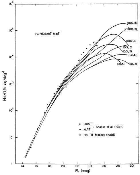
Equally good confirmation of the most basic of the A(m) predictions concerning the gross slope of N(m) as a function of magnitude at the bright end comes from the near-red counts in the IIIa F band. Figure 4 (taken from Figure 9 of Yoshii & Takahara 1988) shows the comparison between observations and the model. The data are from Shanks et al. (1984) and Hall & Mackay (1984).

Figure 4. Same as Figure 3, but for near-red magnitudes in the F-band pass (from Yoshii & Takahara 1988).

Aside from the gross agreement of slopes, Figures 3 and 4 show again the chief result expected earlier (Brown & Tinsley 1974) that the A(m, q₀, E) differential test, or the N(m, q₀, E) integral test, has little hope of finding q₀ because of (a) the first-order insensitivity to the curvature, and (b) the lack of detailed homogeneity due to the sheet and void properties of the distribution, making the test probably impossible even in principle.

The m(z) test (i.e. the Hubble diagram) entirely avoids this latter problem as long as the inhomogeneities do not induce large velocity perturbations on the Hubble flow at high z, which they certainly do not. The upper limit to such perturbations is of the order ~ 500 km s^-1 given by the noncosmological motion of the Local Supercluster relative to the microwave background [see Tammann & Sandage (1985) for a review]; this is a subject for which a large literature now exists (cf. Dressler et al. 1987). Such perturbations at redshifts z ~ 0.5 give velocity perturbations v / v ~ 0.0003, which have negligible effect on m(z), as we now show.