E. Dark energy

The idea that the universe contains close to homogeneous dark energy that approximates a time-variable cosmological "constant" arose in particle physics, through the discussion of phase transitions in the early universe and through the search for a dynamical cancellation of the vacuum energy density; in cosmology, through the discussions of how to reconcile a cosmologically flat universe with the small mass density indicated by galaxy peculiar velocities; and on both sides by the thought that might be very small now because it has been rolling toward zero for a very long time. ⁴⁴

The idea that the dark energy is decaying by emission of matter or radiation is now strongly constrained by the condition that the decay energy must not significantly disturb the spectrum of the 3 K cosmic microwave background radiation. But the history of the idea is interesting, and decay to dark matter still a possibility, so we comment on both here. The picture of dark energy in the form of defects in cosmic fields has not received much attention in recent years, in part because the computations are difficult, but might yet prove to be productive. Much discussed nowadays is dark energy in a slowly varying scalar field. The idea is reviewed at some length here and in even more detail in the Appendix. We begin with another much discussed approach: prescribe the dark energy by parameters in numbers that seem fit for the quality of the measurements.

1. The XCDM parametrization

In the XCDM parametrization the dark energy interacts only with itself and gravity, the dark energy density _X(t) > 0 is approximated as a function of world time alone, and the pressure is written as

(43)

an expression that has come to be known as the cosmic equation of state. ⁴⁵ Then the local energy conservation equation (9) is

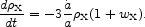(44)

If w_X is constant the dark energy density scales with the expansion factor as

(45)

If w_X < - 1/3 the dark energy makes a positive contribution to /a (Eq. [8]). If w_X = - 1/3 the dark energy has no effect on , and the energy density varies as _X 1 / a², the same as the space curvature term in ² / a² (Eq. [11]). That is, the expansion time histories are the same in an open model with no dark energy and in a spatially-flat model with w_X = - 1/3, although the spacetime geometries differ. ⁴⁶ If w_X < - 1 the dark energy density is increasing. ⁴⁷

Equation (45) with constant w_X has the great advantage of simplicity. An appropriate generalization for the more precise measurements to come might be guided by the idea that the dark energy density is close to homogeneous, spatial variations rearranging themselves at close to the speed of light, as in the scalar field models discussed below. Then for most of the cosmological tests we have an adequate general description of the dark energy if we let w_X be a free function of time. ⁴⁸ In scalar field pictures w_X is derived from the field model; it can be a complicated function of time even when the potential is a simple function of the scalar field.

The analysis of the large-scale anisotropy of the 3 K cosmic microwave background radiation requires a prescription for how the spatial distribution of the dark energy is gravitationally related to the inhomogeneous distribution of other matter and radiation (Caldwell et al., 1998). In XCDM this requires at least one more parameter, an effective speed of sound, with c²_sX > 0 (for stability, as discussed in Sec. II.B), in addition to w_X.

2. Decay by emission of matter or radiation

Bronstein (1933) introduced the idea that the dark energy density is decaying by the emission of matter or radiation. The continuing discussions of this and the associated idea of decaying dark matter (Sciama, 2001, and references therein) are testimony to the appeal. Considerations in the decay of dark energy include the effect on the formation of light elements at z ~ 10¹⁰, the contribution to the -ray or optical extragalactic background radiation, and the perturbation to the spectrum of the 3 K cosmic microwave background radiation. ⁴⁹

The effect on the 3 K cosmic microwave background was of particular interest a decade ago, as a possible explanation of indications of a significant departure from a Planck spectrum. Precision measurements now show the spectrum is very close to thermal. The measurements and their interpretation are discussed by Fixsen et al. (1996). They show that the allowed addition to the 3 K cosmic microwave background energy density _R is limited to just _R / _R 10^-4 since redshift z ~ 10⁵, when the interaction between matter and radiation was last strong enough for thermal relaxation. The bound on _R / _R is not inconsistent with what the galaxies are thought to produce, but it is well below an observationally interesting dark energy density.

Dark energy could decay by emission of dark matter, cold or hot, without disturbing the spectrum of the 3 K cosmic microwave background radiation. For example, let us suppose the dark energy equation of state is w_X = - 1, and hypothetical microphysics causes the dark energy density to decay as a^-n by the production of nonrelativistic dark matter. Then Bronstein's Eq. (36) says the dark matter density varies with time as

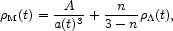(46)

where A is a constant and 0 < n < 3. In the late time limit the dark matter density is a fixed fraction of the dark energy. But for the standard interpretation of the measured anisotropy of the 3 K background we would have to suppose the first term on the right hand side of Eq. (46) is not much smaller than the second, so the coincidences issue discussed in Sec. III.B.2 is not much relieved. It does help relieve the problem with the small present value of (to be discussed in connection with Eq. [47]).

We are not aware of any work on this decaying dark energy picture. Attention instead has turned to the idea that the dark energy density evolves without emission, as illustrated in Eq. (45) and the two classes of physical models to be discussed next.

3. Cosmic field defects

The physics and cosmology of topological defects produced at phase transitions in the early universe are reviewed by Vilenkin and Shellard (1994). An example of dark energy is a tangled web of cosmic string, with fixed mass per unit length, which self-intersects without reconnection. In Vilenkin's (1984) analysis ⁵⁰ the mean mass density in strings scales as _string (ta(t))^-1. When ordinary matter is the dominant contribution to ² / a², the ratio of mass densities is _string / t^1/3. Thus at late times the string mass dominates. In this limit, _string a^-2, w_X = - 1/3 for the XCDM parametrization of Eq. (45), and the universe expands as a t. Davis (1987) and Kamionkowski and Toumbas (1996) propose the same behavior for a texture model. One can also imagine domain walls fill space densely enough not to be dangerous. If the domain walls are fixed in comoving coordinates the domain wall energy density scales as _X a^-1 (Zel'dovich, Kobzarev, and Okun, 1974; Battye, Bucher, and Spergel, 1999). The corresponding equation of state parameter is w_X = - 2/3, which is thought to be easier to reconcile with the supernova measurements than w_X = - 1/3 (Garnavich et al., 1998; Perlmutter et al., 1999a). The cosmological tests of defects models for the dark energy have not been very thoroughly explored, at least in part because an accurate treatment of the behavior of the dark energy is difficult (as seen, for example, in Spergel and Pen, 1997; Friedland, Muruyama, and Perelstein, 2002), but this class of models is worth bearing in mind.

4. Dark energy scalar field

At the time of writing the popular picture for dark energy is a classical scalar field with a self-interaction potential V() that is shallow enough that the field energy density decreases with the expansion of the universe more slowly than the energy density in matter. This idea grew in part out of the inflation scenario, in part from ideas from particle physics. Early examples are Weiss (1987) and Wetterich (1988). ⁵¹ The former considers a quadratic potential with an ultralight effective mass, an idea that reappears in Frieman et al. (1995). The latter considers the time variation of the dark energy density in the case of the Lucchin and Matarrese (1985a) exponential self-interaction potential (Eq. [38]). ⁵²

In the exponential potential model the scalar field energy density varies with time in constant proportion to the dominant energy density. The evidence is that radiation dominates at redshifts in the range 10³ z 10¹⁰, from the success of the standard model for light element formation, and matter dominates at 1 z 10³, from the success of the standard model for the gravitational growth of structure. This would leave the dark energy subdominant today, contrary to what is wanted. This led to the proposal of the inverse power-law potential in Eq. (31) for a single real scalar field. ⁵³

We do not want the hypothetical field to couple too strongly to baryonic matter and fields, because that would produce a "fifth force" that is not observed. ^{54, 55} Within quantum field theory the inverse power-law scalar field potential makes the model non-renormalizable and thus pathological. But the model is meant to describe what might emerge out of a more fundamental quantum theory, which maybe also resolves the physicists' cosmological constant problem (Sec. III.B), as the effective classical description of the dark energy. ⁵⁶ The potential of this classical effective field is chosen ad hoc, to fit the scenario. But one can adduce analogs within supergravity, superstring/M, and brane theory, as reviewed in the Appendix.

The solution for the mass fraction in dark energy in the inverse power-law potential model (in Eq. [33] when << , and the numerical solution at lower redshifts) is not unique, but it behaves as what has come to be termed an attractor or tracker: it is the asymptotic solution for a broad range of initial conditions. ⁵⁷ The solution also has the property that is decreasing, but less rapidly than the mass densities in matter and radiation. This may help alleviate two troubling aspects of the cosmological constant. The coincidences issue is discussed in Sec. III.B. The other is the characteristic energy scale set by the value of ,

(47)

when _R0 and _K0 may be neglected. In the limit of constant dark energy density, cosmology seems to indicate new physics at an energy scale more typical of chemistry. If is rolling toward zero the energy scale might look more reasonable, as follows (Peebles and Ratra, 1988; Steinhardt et al., 1999; Brax et al., 2000).

Suppose that as conventional inflation ends the scalar field potential switches over to the inverse power-law form in Eq. (31). Let the energy scale at the end of inflation be (t_I) = (t_I)^1/4, where (t_I) is the energy density in matter and radiation at the end of inflation, and let (t_I) be the energy scale of the dark energy at the end of inflation. Since the present value (t₀) of the dark energy scale (Eq. [47]) is comparable to the present energy scale belonging to the matter, we have from Eq. (33)

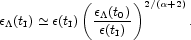(48)

For parameters of common inflation models, (t_I) ~ 10¹³ GeV, and (t₀) / (t_I) ~ 10^-25. If, say, = 6, then

(49)

As this example illustrates, one can arrange the scalar field model so it has a characteristic energy scale that exceeds the energy ~ 10³ GeV below which physics is thought to be well understood: in this model cosmology does not force upon us the idea that there is as yet undiscovered physics at the very small energy in Eq. (47). Of course, where the factor ~ 10^-6 in Eq. (49) comes from still is an open question, but, as discussed in the Appendix, perhaps easier to resolve than the origin of the factor ~ 10^-25 in the constant case.

When we can describe the dynamics of the departure from a spatially homogeneous field in linear perturbation theory, a scalar field model generally is characterized by the time-dependent values of w_X (Eq. [43]) and the speed of sound c_sX (e.g., Ratra, 1991; Caldwell et al., 1998). In the inverse power-law potential model the relation between the power-law index and the equation of state parameter in the matter-dominated epoch is independent of time (Ratra and Quillen, 1992),

(50)

When the dark energy density starts to make an appreciable contribution to the expansion rate the parameter w_X starts to evolve. The use of a constant value of w_X to characterize the inverse power-law potential model thus can be misleading. For example, Podariu and Ratra (2000, Fig. 2) show that, when applied to the Type Ia supernova measurements, the XCDM parametrization in Eq. (50) leads to a significantly tighter apparent upper limit on w_X, at fixed _M0, than is warranted by the results of a computation of the evolution of the dark energy density in this scalar field model. Caldwell et al. (1998) deal with the relation between scalar field models and the XCDM parametrization by fixing w_X, as a constant or some function of redshift, deducing the scalar field potential V() that produces this w_X, and then computing the gravitational response of to the large-scale mass distribution.

⁴⁴ This last idea is similar in spirit to Dirac's (1937, 1938) attempt to explain the large dimensionless numbers of physics. He noted that the gravitational force between two protons is much smaller than the electromagnetic force, and that that might be because the gravitational constant G is decreasing in inverse proportion to the world time. This is the earliest discussion we know of what has come to be called the hierarchy problem, that is, the search for a mechanism that might be responsible for the large ratio between a possibly more fundamental high energy scale, for example, that of grand unification or the Planck scale (where quantum gravitational effects become significant) and a lower possibly less fundamental energy scale, for example that of electroweak unification (see, for example, Georgi, Quinn, and Weinberg, 1974). The hierarchy problem in particle physics may be rephrased as a search for a mechanism to prevent the light electroweak symmetry breaking Higgs scalar field mass from being large because of a quadratically divergent quantum mechanical correction (see, for example, Susskind, 1979). In this sense it is similar in spirit to the physicists' cosmological constant problem of Sec. III.B. Back.

⁴⁵ Other parametrizations of dark energy are discussed by Hu (1998) and Bucher and Spergel (1999). The name, XCDM, for the case w_X < 0 in Eq. (43), was introduced by Turner and White (1997). There is a long history in cosmology of applications of such an equation of state, and the related evolution of ; examples are Canuto et al. (1977), Lau (1985), Huang (1985), Fry (1985), Hiscock (1986), Özer and Taha (1986), and Olson and Jordan (1987). See Ratra and Peebles (1988) for references to other early work on a time-variable and Overduin and Cooperstock (1998) and Sahni and Starobinsky (2000) for reviews. More recent discussions of this and related models may be found in John and Joseph (2000), Zimdahl et al. (2001), Dalal et al. (2001), Gudmundsson and Björnsson (2002), Bean and Melchiorri (2002), Mak, Belinchón, and Harko (2002), and Kujat et al. (2002), through which other recent work may be traced. Back.

⁴⁶ As discussed in Sec. IV, it appears difficult to reconcile the case w_X = - 1/3 with the Type Ia supernova apparent magnitude data (Garnavich et al., 1998; Perlmutter et al., 1999a). Back.

⁴⁷ This is quite a step from the thought that the dark energy density is small because it has been rolling to zero for a long time, but the case has found a context (Caldwell, 2002; Maor et al., 2002). Such models were first discussed in the context of inflation (e.g., Lucchin and Matarrese, 1985b), where it was shown that the w_X < - 1 component could be modeled as a scalar field with a negative kinetic energy density (Peebles, 1989a). Back.

⁴⁸ The availability of a free function greatly complicates the search for tests as opposed to curve fitting! This is clearly illustrated by Maor et al. (2002). For more examples see Perlmutter, Turner, and White (1999b) and Efstathiou (1999). Back.

⁴⁹ These considerations generally are phenomenological: the evolution of the dark energy density, and its related coupling to matter or radiation, is assigned rather than derived from an action principle. Recent discussions include Pollock (1980), Kazanas (1980), Freese et al. (1987), Gasperini (1987), Sato, Terasawa, and Yokoyama (1989), Bartlett and Silk (1990), Overduin, Wesson, and Bowyer (1993), Matyjasek (1995), and Birkel and Sarkar (1997). Back.

⁵⁰ The string flops at speeds comparable to light, making the coherence length comparable to the expansion time t. Suppose a string randomly walks across a region of physical size a(t)R in N steps, where aR ~ N^1/2t. The total length of this string within the region R is l ~ Nt. Thus the mean mass density of the string scales with time as _string l / a³ (ta(t))^-1. One randomly walking string does not fill space, but we can imagine many randomly placed strings produce a nearly smooth mass distribution. Spergel and Pen (1997) compute the 3 K cosmic microwave background radiation anisotropy in a related model, where the string network is fixed in comoving coordinates so the mean mass density scales as _string a^-2. Back.

⁵¹ Other early examples include those cited in Ratra and Peebles (1988) as well as Endo and Fukui (1977), Fujii (1982), Dolgov (1983), Nilles (1985), Zee (1985), Wilczek (1985), Bertolami (1986), Ford (1987), Singh and Padmanabhan (1988), and Barr and Hochberg (1988). Back.

⁵² For recent discussions of this model see Ferreira and Joyce (1998), Ott (2001), Hwang and Noh (2001), and references therein. Back.

⁵³ In what follows we focus on this model, which was proposed by Peebles and Ratra (1988). The model assumes a conventionally normalized scalar field kinetic energy and spatial gradient term in the action, and it assumes the scalar field is coupled only to itself and gravity. The model is then completely characterized by the form of the potential (in addition to all the other usual cosmological parameters, including initial conditions). Models based on other forms for V(), with a more general kinetic energy and spatial gradient term, or with more general couplings to gravity and other fields, are discussed in the Appendix. Back.

⁵⁴ The current value of the mass associated with spatial inhomogeneities in the field is m(t₀) ~ H₀ ~ 10^-33 eV, as one would expect from the dimensions. More explicitly, one arrives at this mass by writing the field as (t, ) = <>(t) + (t, ) and Taylor expanding the scalar field potential energy density V() about the homogeneous mean background <> to quadratic order in the spatially inhomogeneous part , to get m² = V"(<>). Within the context of the inverse power-law model, the tiny value of the mass follows from the requirements that V varies slowly with the field value and that the current value of V be observationally acceptable. The difference between the roles of m and the constant m_q in the quadratic potential model V = m_q^{2 2} / 2 is worth noting. The mass m_q has an assigned and arguably fine-tuned value. The effective mass m ~ H belonging to V ^- is a derived quantity, that evolves as the universe expands. The small value of m(t₀) explains why the scalar field energy cannot be concentrated with the non-relativistic mass in galaxies and clusters of galaxies. Because of the tiny mass a scalar field would mediate a new long-range fifth force if it were not weakly coupled to ordinary matter. Weak coupling also ensures that the contributions to coupling constants (such as the gravitational constant) from the exchange of dark energy bosons are small, so such coupling constants are not significantly time variable in this model. See, for example, Carroll (1998), Chiba (1999), Horvat (1999), Amendola (2000), Bartolo and Pietroni (2000), and Fujii (2000) for recent discussions of this and related issues. Back.

⁵⁵ Coupling between dark energy and dark matter is not constrained by conventional fifth force measurements. An example is discussed by Amendola and Tocchini-Valentini (2002). Perhaps the first consideration is that the fifth-force interaction between neighboring dark matter halos must not be so strong as to shift regular galaxies of stars away from the centers of their dark matter halos. Back.

⁵⁶ Of course, the zero-point energy of the quantum-mechanical fluctuations around the mean field value contributes to the physicists' cosmological constant problem, and renormalization of the potential could destroy the attractor solution (however, see Doran and Jäckel, 2002) and could generate couplings between the scalar field and other fields leading to an observationally inconsistent "fifth force". The problems within quantum field theory with the idea that the energy of a classical scalar field is the dark energy, or drives inflation, are further discussed in the Appendix. The best we can hope is that the effective classical model is a useful approximation to what actually is happening, which might lead us to a more satisfactory theory. Back.

⁵⁷ A recent discussion is in Brax and Martin (2000). Brax, Martin, and Riazuelo (2000) present a thorough analysis of the evolution of spatial inhomogeneities in the inverse power-law scalar field potential model and confirm that these inhomogeneities do not destroy the homogeneous attractor solution. For other recent discussions of attractor solutions in a variety of contexts see Liddle and Scherrer (1999), Uzan (1999), de Ritis et al. (2000), Holden and Wands (2000), Baccigalupi, Matarrese, and Perrotta (2000), and Huey and Tavakol (2002). Back.