


2.1. Modelling galaxies and their Stellar Populations, a Historical Introduction
The stellar mass M* of a galaxy is a key physical parameter of galaxy formation and evolution studies as it traces the galaxy formation process. The stellar mass of a galaxy grows through processes such as the internal conversion of gas and dust into stars via star formation, or external events like major interactions with other galaxies and subsequent merging which may induce further star formation, as well as minor events such as accretion of satellites. Moreover, knowledge of the galaxy stellar mass is crucial in order to decompose the contributions from stars and dark matter to the dynamics of galaxies. Modern galaxy formation models embedded in a Λ-Cold Dark Matter universe can also predict the evolution of the galaxy mass assembly over cosmic time (e.g. De Lucia et al. 2007).
Galaxies shine because their stars radiate the energy they produced via nuclear reactions in their cores. The theory of stellar evolution describes the amount of energy released by a star given its initial mass. Hence, by modelling the light emitted by all the stars in a galaxy over all wavelengths - the so-called "integrated spectral energy distribution (SED)" - one can in principle derive the stellar mass that is responsible for such radiation. However, a certain fraction of evolved stars no longer shine yet still contribute to the galaxy mass budget in the form of stellar remnants such as white dwarfs, neutron stars and black holes. The sum of living stars plus remnants makes up the "stellar mass", M*, of a galaxy.
Despite our detailed knowledge of stellar evolution, the modelling of a galaxy spectrum - which is the superposition of all spectra from individual stars - is a challenging exercise since the exact stellar composition of a galaxy and its overall stellar generations are unknown a priori. These depend on the history of star formation, chemical enrichment, accretion and interaction. Unlike stellar clusters whose vast majority of stars are coeval and share the same chemical composition, galaxies are a complicated ensemble of stellar generations. Recent extensive reviews of SED modelling of galaxies have appeared in Walcher et al. (2011) and Conroy (2013).
As recognised early on by Oort (1926) and Baade (1944), our own Milky Way is composed of various populations of stars, each featuring different dynamics, chemical properties, and formation epochs. Thus, from a stellar content viewpoint, galaxies can be broken into stellar populations with shared definable properties. The "simple stellar population" (SSP) is defined as a group of coeval stars with homogeneous chemistry (at birth) and similar orbits/kinematics. A recent, comprehensive text book on stellar populations in galaxies is due to Greggio & Renzini (2011).
Star clusters, either open or globular, are the closest realisation of SSPs in nature. The main unknown of an SSP is the stellar Initial Mass Function (IMF), which gives the mass spectrum of the stellar generation at birth. The latter is not known from first principles. Empirical determinations of the IMF based on solar neighborhood data were first modeled by Salpeter (1955) as a power-law with exponent of ~ -2.35. An IMF must be assumed when calculating the properties of population models. While galaxies are not SSPs, they can be viewed as a sum of all present SSPs: that is, Galaxies = ∑j SSPj . The distribution of stellar generations in time and chemical enrichment is called the "Star Formation History" (SFH). Several analytical laws describe plausible SFHs which depend on the timescale of the Star Formation Rate (SFR), such as exponentially-declining models, or τ-models, models with constant star formation, models with time-increasing star formation, etc. Examples of such SFHs are shown in Figure 1.
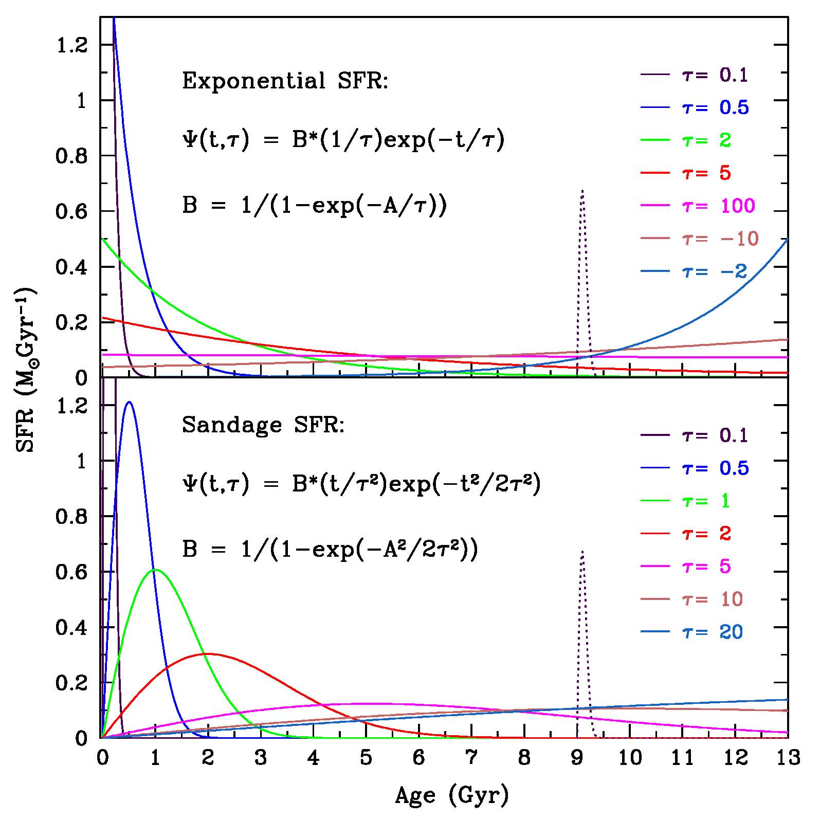 |
Figure 1. Time evolution of the exponential (upper panel) and Sandage (1986a) (lower panel) star formation histories (solid curves). The dotted curve is a Sandage-style burst of star formation in which 10% of the total mass of stars are formed. From MacArthur et al. (2004). |
Ultimately, the stellar content of a galaxy over time, t, may be thought of as:
 |
(1) |
with Y the Helium abundance and Z the abundance of heavier elements (metallicity). Note that Y, Z, and the IMF may vary between different stellar generations, i.e. amongst different SSPs, but they do not vary within an SSP by definition.
It is useful to note that little is known about the physical processes that drive the rate of star formation and the emerging mass spectrum (the IMF). We know that stars form from dense, cold gas in gas that is shock compressed (e.g. in disks, during galaxy interactions or dynamical instabilities), but a theory which predicts the SFR and the IMF in different galaxies and as a function of time has yet to be written. For these reasons, these two physical quantities are parametrized in population models and observations to guide ongoing developments. Indeed, our limited knowledge about the SFR and IMF is a major problem in the precise determination of a galaxy's stellar mass.
Historically, the problem of modelling a galaxy spectrum has been approached in two ways. In the so-called "optimised population synthesis" (Spinrad & Taylor 1971; Faber 1972; O'Connell 1976; Pickles 1985; Bica & Alloin 1986), empirical stellar spectra are combined in proportions such that the resulting composite spectrum can best reproduce the galaxy spectrum. These proportions can be ad hoc, hence neither necessarily obeying stellar evolution timescales nor a realistic stellar IMF. The obtained best-fit model can provide an excellent representation of the galaxy spectrum, but it cannot be evolved with time. Hence the optimised spectral fitting does not allow to study galaxy evolution in a cosmological context. Still, it can provide important insights on the types of stars which are effectively present in a stellar system (e.g. MacArthur et al. 2009). Optimised synthesis can also be used to obtain an instantaneous description of a galaxy spectrum in order to achieve accurate estimates of broadening of absorption lines for velocity dispersion measurements (see Section 5).
The alternative approach makes use of stellar evolutionary models, which describe the detailed time evolution of the luminosity and temperature of stars of different mass. Integrated spectra for galaxies are calculated by adding up the contributions of the individual model stars after assuming an IMF and a SFH. These so-called "evolutionary population synthesis models", based on stellar evolution theory, can be evolved in time back and forth and galaxy evolution can be studied at arbitrary cosmic distances with the same underlying theory. The comparison between these models and observational data provides estimates for the average formation epoch, metallicity and SFH of a galaxy, thus enabling an evaluation of the stellar mass through the model mass-to-light, or M* / L, ratio. These models, pioneered by Tinsley (1972), Tinsley & Gunn (1976), Renzini & Voli (1981), and Bruzual (1983), from which galaxy stellar masses are derived, will be described extensively in the next section (Section 2.2), focusing on the quantities that affect directly the stellar mass derivation, using various models available in the literature. We also address the impact of different model fitting techniques on extracted results and conclude with an assessment of the accuracy of galaxy stellar mass estimates.
2.2. Basics of Stellar Population Models
Evolutionary Population Synthesis (EPS) models provide the expected spectral energy distribution (SED) of a stellar population as a function of key parameters, such as:
These are the main parameters controlling the time evolution of the population. Further assumptions need to be made for stars evolving over specific evolutionary phases, which will be mentioned below.
The model ingredients are: the stellar evolutionary tracks and/or isochrones, the stellar spectral libraries, the parametrization for the mass-loss which affects several late stages of evolution such as the Thermally-Pulsing Asymptotic Giant Branch (TP-AGB), the Red Giant Branch (RGB), the Horizontal Branch (HB), and also the Main Sequence (MS) in young populations.
A further model feature is the computational procedure, which may be an integration by mass of the luminosity contributions (so-called isochrone synthesis technique, Bruzual & Charlot 1993) or a technique based on Renzini's fuel consumption theorem (Renzini 1981; Buzzoni 1989; Maraston 1998; 2005). This theorem states that the number of stars at each burning stage is proportional to the time it takes to exhaust the nuclear fuel burnt at that stage. This can be interpreted as the conservation of energy for stellar populations. In population synthesis models, it is a useful tool to quantify the contribution of rapid, and very luminous, stellar phases as found at the tip of the RGB, the AGB and the RGB bump cf. discussion in Maraston (2005). Numerical experiments have shown that calculations based on the fuel consumption theorem and isochrone synthesis agree well (Charlot & Bruzual 1991), provided the mass bin of the mass integration in the isochrone synthesis case is small (Maraston 1998 finds 10-6 M⊙ for the tip of the RGB). Moreover, the fuel consumption theorem is useful for including in synthetic integrated models those stellar phases for which a complete isochrone may not be available, such as the AGB, the Horizontal Branch with different morphologies, and the hot stars responsible for producing the UV-upturn in ellipticals.
A detailed description of the individual population models can be found in the corresponding papers, e.g. Vazdekis et al. (1996, hereafter, Vazdekis models), Fioc & Rocca-Volmerange (1997, PEGASE models), Bruzual & Charlot (2003, BC03), Maraston (2005, Maraston) and Conroy et al. (2009, FSPS), in addition to the reviews cited in the previous section.
The basic model EPS unit is the SSP. In the following SSPs are first used to illustrate the fundamental dependencies of M* / L on age and metallicity, with composite models treated later on.
The most important driver of an SSP's luminosity evolution is its
age, since the most massive stars live quickly but are orders of
magnitude more luminous than smaller mass stars. For most IMFs the mass
of a stellar population
is dominated by the faintest stars and changes relatively
little with time after the first Gyr of age (see
Figure 2),
but the luminosity of a population is dominated by its brightest stars
showing large changes over time. Besides the Main Sequence, which
provides a substantial contribution to the light at virtually every
age, the brightest stars are found in different post-Main Sequence (PMS)
evolutionary phases. Which phase dominates depends upon the age of the
stellar population and the wavelength of observation.
In young populations (t
 200 Myr),
Helium burning stars dominate the light, while at intermediate-age
(200 Myr < t
2 Gyr), the
Thermally-Pulsing Asymptotic
Giant Branch (TP-AGB) stars take over (in some models, see below); at old
ages, Red Giant Branch (RGB) stars outshine all other stars.
AGB and RGB phases are mostly bright in the near-IR (NIR), while MS stars
contribute mostly to optical bands see Fig. 11 in
Maraston (1998).
200 Myr),
Helium burning stars dominate the light, while at intermediate-age
(200 Myr < t
2 Gyr), the
Thermally-Pulsing Asymptotic
Giant Branch (TP-AGB) stars take over (in some models, see below); at old
ages, Red Giant Branch (RGB) stars outshine all other stars.
AGB and RGB phases are mostly bright in the near-IR (NIR), while MS stars
contribute mostly to optical bands see Fig. 11 in
Maraston (1998).
 |
Figure 2. The stellar bolometric M* / L and M* / L in various bands (B, V, K) as function of age for SSPs (single burst models) and the different indicated metallicities. All models for Kroupa IMF, except for the thin solid line in the top left diagram for a Salpeter IMF. The stellar mass M* in this figure accounts for stellar mass losses, as in Maraston (1998; 2005). See also text for details. From Maraston (2005). |
The luminosity of an SSP is therefore a strong function of time.
This rate varies with wavelength given the contributions from different
evolutionary phases. The overall luminosity evolution is more significant
in the blue/optical spectral range where MS stars dominate, scaling roughly
logarithmically with time
(Tinsley 1972),
as compared to the NIR light of old populations (t
 2-3 Gyr), where
the slowly evolving
RGB stars dominate. The rate of luminosity change at NIR wavelengths
is large near 0.3-1 Gyr in models including the TP-AGB phase (e.g.
Maraston 1998;
Maraston 2005;
Marigo et
al. 2008),
since the onset of
this phase implies a rapid increase of the NIR luminosity due to the
cool and luminous TP-AGB stars. This effect is model-dependent. Global
age and metallicity effects on the M* / L in
various bands for SSP models is shown in Figure 2.
2-3 Gyr), where
the slowly evolving
RGB stars dominate. The rate of luminosity change at NIR wavelengths
is large near 0.3-1 Gyr in models including the TP-AGB phase (e.g.
Maraston 1998;
Maraston 2005;
Marigo et
al. 2008),
since the onset of
this phase implies a rapid increase of the NIR luminosity due to the
cool and luminous TP-AGB stars. This effect is model-dependent. Global
age and metallicity effects on the M* / L in
various bands for SSP models is shown in Figure 2.
The stellar population's metallicity also affects stellar evolution time scales and mostly the stellar SEDs. Metal-rich stars are cooler (because of a higher opacity in their stellar envelopes) and fainter (because the turnoff mass is smaller and most outgoing photons are trapped into their envelope), hence the higher M* / L of a metal-rich population due to a lower luminosity (while M* changes little). This trend is visible in Figure 2. Metallicity effects are significantly milder at NIR bandpasses; at very high metallicity (see the 3.5 solar metallicity track in Figure 2, long dashed line), the trend reverses in NIR bands, since the luminosity of such a metal-enriched population is concentrated at longer wavelengths see Maraston (2005, for a full discussion). As is well known, ageing of a stellar population has the same effect as increasing metals since, as the most massive stars die out, the temperature distribution skews towards cooler values. The combined age and metallicity effects on dwarf and giant stars result in the so-called "age-metallicity (A/Z) degeneracy" in the optical region of their spectrum (e.g. Faber 1972; Renzini & Buzzoni 1986; Worthey 1994; Maraston & Thomas 2000). At optical wavelengths, the effect is such that a population of stars that is three times more metal rich mimics a population twice its age; this is the "3/2 rule" of Worthey (1994). This A/Z degeneracy at optical wavelengths obviously holds for M* / L ratios as well. The optical A/Z degeneracy can be lifted by including data at longer wavelengths where giants dominate the spectrum and increasing metallicity results in redder colors, with a small dependence on age (with the exception of the AGB time). Worthey (1994) proposed that the spectral region around 1 micron (i.e. between the I,J bandpasses, depending slightly on age and IMF) is the most insensitive to metallicity. This notion has been exploited with color-color diagrams involving optical and at least one NIR passbands to analyse the stellar populations of integrated stellar systems (e.g. de Jong 1996; Bell & de Jong 2000; Maraston et al. 2001; MacArthur et al. 2004; Roediger et al. 2011). This concept of using an extended wavelength range has also been exploited for the study of high-redshift galaxies where the time spanned since the Big Bang is short and the age dependencies can be disregarded. In particular, the TP-AGB phase appears in galaxy spectra and the inclusion of the NIR allows galaxy ages to be better constrained (Maraston et al. 2006).
 |
Figure 3. Evolution of the stellar mass fractions for stellar populations with the same total initial mass (normalized to 1 M⊙) and different initial mass functions. "Bottom-Heavy" and "Top-Heavy" are extreme cases of single-sloped IMFs with exponents 3.5 and 1 in the notation in which the Salpeter slope is 2.35. M* evolves because stars die progressively and leave remnants with mass lower than the initial mass. Also shown are the fractions of M* in remnants, namely White Dwarfs (WD), Neutron Stars (NS) and Black Holes (BH). Based on Maraston (2005) models. |
The total stellar mass M* of an SSP also evolves with time. It typically decreases with time since the most massive stars progressively die leaving stellar remnants with mass smaller than the initial ones. M* is a strong function of the IMF. Figure 3 shows the evolution of M* for several widely-used empirically-based IMFs, namely Salpeter (1955, black), Kroupa (2001, red), Chabrier (2003, green). These IMFs follow the same Salpeter power law slope for stellar masses larger than 0.6 M⊙, but have, to varying degrees, less stars than predicted by this Salpeter law slope below this mass limit (hence bottom-light). It should be reminded that Salpeter (1955, black), Kroupa (2001, red), Chabrier (2003, green) were all based on solar neighborhood data.
Also shown are two additional, not empirically-based IMFs meant to illustrate extreme cases of a dwarf-dominated (labeled "bottom-heavy") and a giant-dominated (labeled "top-heavy") IMF. These are single-sloped IMFs with exponents 3.5 and 1 in the notation in which the Salpeter's one is 2.35, and are meant to illustrate galaxies dominated by low-mass and high-mass stars, respectively. Evidence for these extreme IMFs has been advocated in the literature. For example, van Dokkum & Conroy (2012) suggest a dwarf-dominated IMF in massive early-type galaxies (hereafter ETGs) to explain the strength of near-IR lines. Similarly, dynamical modeling studies Cappellari et al. (2012, see also Section 5) and gravitational lensing studies (Treu et al. 2010; Auger et al. 2010b; Brewer et al. 2012, see also Section 7) of ETGs find evidence for the same type of IMF, with larger mass-to-light ratios than those predicted by Chabrier-like IMFs.
At the other end of the mass spectrum, Baugh et al. (2007) find that a top-heavy IMF in high-redshift bursts helps in explaining the colours of massive dusty and bursty distant galaxies (so-called "sub-millimiter" galaxies).
For the same total initial mass, the stellar masses of top-heavy IMFs evolve faster with time because of their larger proportion of massive stars. Most of the evolution occurs within the first Gyr, following the much faster evolution timescales of stars more massive than roughly 2 M⊙. Over a Hubble time, the amount of mass loss averages 30 to 40% of the initial mass. For composite population models with ongoing star formation, the decrement is reduced to ~ 20% (see Maraston et al. 2006). In the Maraston models, the total remnant mass is budgeted amongst white dwarfs, neutron stars and black holes, following the analytical prescription of Renzini & Ciotti (1993). Maraston (1998) has explored IMFs with various exponents to show that M* is maximally large for both dwarf-dominated as well as top-heavy IMFs, while the minimum M* is achieved with a bottom-light 2. IMFs such as the Scalo (1986), Kroupa (2001) or Chabrier (2003)-type IMFs (see Figs 16, 17 in Maraston 1998). A population born with a dwarf-dominated (or "bottom-heavy") IMF has a large M* since most stars have a small mass hence their extended lifetime and they contribute their total mass to M*. A giant-dominated (or "top-heavy") IMF has a large M* given by the large number of massive remnants left by the evolved massive stars. These considerations are important as the value of M* and the assumptions regarding the IMF impact directly the evaluation of the total stellar mass and the dark matter content in galaxies.
It should be noted that the predicted M* may differ amongst different population synthesis models (see model comparisons between Bruzual & Charlot 2003 and Maraston 2005 in Fig. 3 of MacArthur et al. 2010). This discrepancy may reflect a different accounting of stellar remnants. Hence, in comparing stellar masses obtained with different EPS models, one should also consider if and how the remnant masses are accounted for. For example, the Worthey (1994) models consider the mass contribution of the sole living stars, while Bruzual & Charlot (1993) consider a constant M*, etc.
Other factors may complicate the broad-brush stellar evolution picture painted above. For example, stars in exotic evolutionary phases - such as Hot Horizontal Branch (HHB) at high metallicity and Blue Straggler (BS) stars - may alter the luminosity in the blue spectral range. These events probably affect mostly globular cluster studies, as the relative contribution of these phases to the total light of a galaxy should not be very significant. Also, one should not rely on a single band - especially a blue band - to determine stellar masses. The reddest side of the spectrum is equally challenging with the evolution along the TP-AGB being woefully uncertain due to the unknown mass loss. A lively debate pertaining to the reliability of optical/NIR stellar mass estimates is currently ongoing (e.g., Bruzual 2007, Marigo et al. 2008, Conroy et al. 2009, Zibetti et al. 2009, MacArthur et al. 2010, Conroy & Gunn 2010, Lyubenova et al. 2012, and Conroy 2013).
A resolution of the significance of the TP-AGB phase to stellar mass estimates cannot be achieved in this review. However, a sound estimate of the stellar mass appears to be provided by the g-r color (Zibetti et al. 2009; Taylor et al. 2011). The effect of the TP-AGB phase on stellar mass derivations stemming from the use of models with and without a substantial TP-AGB contribution is highlighted when appropriate.
Extinction from dust also affects broadband luminosities hence M* / L ratios and stellar population colors. However, in optical passbands the expected dust effects on M* / L and population color run parallel to the expected stellar population color-M* / L relations and the mass estimates are only weakly affected (e.g. Bell & de Jong 2001). Likewise, line indices are only slightly affected by dust (MacArthur 2005) and can help disentangle extinction from population effects. For full stellar mass estimation dust extinction should be included in analyses, but dust is here not further addressed. Finally, most stellar systems will not be approximated by single-burst or SSP models, rather by composite populations with multiple ages and metallicities. The unknown galaxy star formation histories complicate the interpretation of integrated light observations and will be discussed in Section 2.3.1).
In the following we focus on mass determinations in relation to fitting of the broad-band spectrum, as this situation is common to both low as well as high-redshift studies, where high resolution spectral fitting is presently unfeasible. It should also be noticed that comparison of galaxy mass determinations obtained via broad-band or spectral fitting agree well when the signal-to-noise of the spectrum is high (Chen et al. 2012).
2.3. Stellar Mass from M* / L vs Colour Diagnostics
The list at the beginning of Section 2.2 makes clear that the "Big 4" variables that stand between the observed photometric distribution of star-light and our interpretation in terms of stellar mass are: (i) the correctness of stellar evolution models along stellar phases; (ii) the SFH; (iii) the chemical enrichment history; and (iv) the IMF. These are all inter-connected astrophysically and phenomenologically. Part of this interconnection could be labeled the 5th variable of "environment". In most cases when analysing galaxies, little information is available on the big 4, with perhaps the exclusion of (i) which can be calibrated and tested in local stars. Hence, usually a variety of models are assumed including different formalizations for (ii), (iii) and (iv). The significance of these assumptions is shown below.
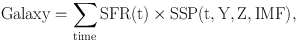
Following Bell & de Jong (2001), we illustrate how M* / L ratios in the B and the K-band correlate with (B-R) and (I-K) colors (as tracers of age and/or metallicity), and the mostly age sensitive HδA index. Figure 2 shows that M* / L values in other optical passbands behave similarly as the M / LB plots, just with a slightly different slope.
Figure 4 shows grids of model colors, M* / L and a spectroscopic index for SSPs of various ages and metallicities. Once a population is older than about 0.1 Gyr, M* / LB versus (B-R) displays a good correlation, which is fairly independent of metallicity. The M* / LK versus (B-R) is more ambiguous with age as M* / LK evolves slowly after the TP-AGB phase-transition (meaning, after some Gyr of age). The relations of M* / L with (I-K) color cannot be used alone to derive M* because the model loci are nearly vertical after 0.1 Gyr, meaning that at a given metallicity M* / L is nearly independent of color. As mentioned earlier, the luminosity in the NIR after a few 100 Myr is dominated by evolved (AGB and later RGB) stars. The lower NIR M* / L at early ages (~ 10 Myr) is due to short-lived, bright red supergiants. Note that this caveat is only relevant for very recent star formation, basically from HII regions.
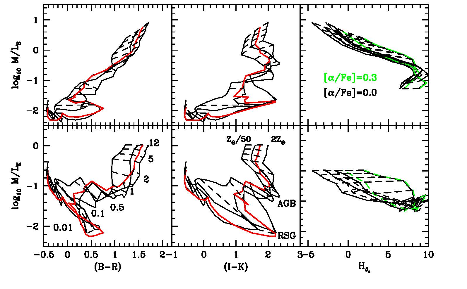 |
Figure 4.Trends of Maraston (2005) SSP models with various ages and metallicities, and a Salpeter IMF. M* / L values in B and K-band (top-to-bottom) are shown versus (B - R), (I - K), and the HδA line index (left-to-right). The latter models are from Thomas et al. (2011a); green lines connect models for [α/Fe] ratio of +0.3, black lines connect solar-scaled models. Models with a same age (in Gyr) are connected with dashed lines, models with a same metallicity with solid lines (Z = 0.001, 0.01, 0.02, 0.04). Red lines highlight solar metallicity (Z = 0.02). |
Perhaps the best approach to measuring M* / L is to fit SEDs simultaneously in at least three passbands, with one in the NIR, hence breaking the age-metallicity degeneracy. Modulo model uncertainties as detailed in the following sections, convergence to the right M* / L value may be achieved (as shown by Zibetti et al. 2009 or by Maraston et al. 2001 for massive star clusters and Maraston et al. 2006 for high-redshift galaxies).
Finally, the rightmost column of Figure 4 shows an example of M* / L trends with an absorption line index. The HδA Balmer line index (Worthey & Ottaviani 1997) was chosen as it has been used specifically for the estimation of M* for the SDSS galaxies (e.g. Kauffmann et al. 2003). This index is sensitive to the age of the stellar population, being the strongest around 0.3-0.5 Gyr (depending on metallicity) when A-type stars dominate the spectrum, and smaller at both older and younger ages (see Fig. 8 in Maraston et al. 2001). This degeneracy for HδA can obviously be broken (for a single burst population) by using an extra spectral indicator with a monotonic behavior with age. Two further complications should be noted. Because of its temperature dependence, the index is also affected by old, though hot, stars such as metal-poor blue HB stars (Maraston et al. 2003). Moreover, the index has been shown to be sensitive to the [α/Fe] ratio, because of strong Fe lines present in the pseudo-continua (Thomas et al. 2004a). For instance, the index is stronger in [α/Fe]-enhanced populations (such as those of massive ETGs) than in solar-scaled ones. The trend with abundance ratios is shown in Figure 4, where the grid in green displays models for the same total metallicity Z, but enhanced [α/Fe] = 0.3. The consideration of these effects when dealing with massive galaxies is important, as a strong index can otherwise only be explained by a lower age, which in turn would induce a mismatch in the derivation of the M* / L ratio. Ideally in the future it should be possible to complete the last panel of Figure 4 by considering the abundance-ratio effects on colors and mass-to-light. Broadbrush, the model grid distribution shown in HδA versus M* / L is similar to the (B-R) versus M* / L distributions, except for the very youngest ages. The same degeneracies are therefore also present in composite age models and we will no longer show the HδA models separately.
Single burst models are ideal cases that apply well to star clusters, but not to galaxies, where a prolonged star formation is in general more appropriate. The determination of M* in these cases is much more difficult, as the latest generations dominate the light and drive down the M* / L hence M*, which leads to underestimate of the stellar mass (Bell & de Jong 2001; MacArthur et al. 2009; Maraston et al. 2010.) These issues are discussed in the next section.
2.3.1. Effect of Star Formation History
Stellar systems like galaxies are expected to have a wide range of SFHs. The effect of prolonged star formation history on the model grids is visualised in Figure 5 by using exponentially declining SFR models or τ-models (as introduced by Bruzual 1983), with SFR(t) ∝ exp(-t/τ), where τ indicates the e-folding timescale of star formation and can be both positive and negative. This model is a reasonable first approximation of the star formation history of a spiral galaxy or, for very low τ's, of a passive system. Negative τ values represent galaxies which have increasing SFRs, especially galaxies with recent star bursts (e.g. Bell & de Jong 2000).
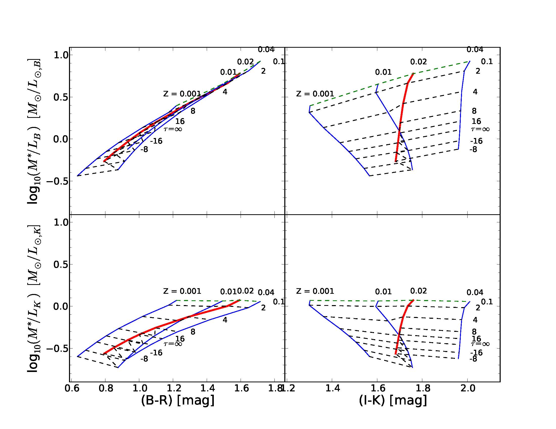 |
Figure 5. Trends in M* / L ratios using exponentially declining star formation rate models. The models are the same as in Figure 4, except that instead of a single burst an exponentially declining star formation rate is used observed at age 12 Gyr after star formation began. Models with the same e-folding timescale τ are connected with dashed lines, where positive τ stands for decreasing star formation rate with time, negative τ for increasing star formation rate, and τ = ∞ is a constant star formation rate model. Solid lines connect models with equal indicated metallicity, where the red line highlights solar metallicity. Based on Maraston (2005) models. |
The model M* / L ratios in the optical are nearly degenerate versus (B-R) in Figure 5. This degeneracy is somewhat broken in (B-R) versus the near-IR M* / LK, especially for the lowest metallicities (Z < 0.004). However, realizing that chemical evolution caused by modest amounts of star formation raises the system metallicity rapidly to at least 0.1 solar (or Z = 0.002; in a closed box, conversion of ~ 20% of gas mass into stars raises the average metallicity to over 0.1 solar), the range of relevant metallicities becomes narrower in most applications, making the color-M* / LK relation tighter.
Tracing mainly evolved stellar populations, (I-K) is largely metallicity sensitive, weakly sensitive on age, and (I-K) on its own (without any other passbands) is not useful for mass estimation as Figure 5 clearly shows. Moreover, the details of evolved stellar evolution stages are still relatively poorly modeled and the exact shapes of these (I-K) diagrams are highly dependent on models used, as shown in Section 2.3.3.
Not all stellar systems are ~12 Gyr old, either because they are observed at higher redshift when the Universe was much younger or because they may have had their major epoch of star formation significantly delayed. The effect of a younger final age on exponential SFR models is shown in Figure 6. This figure shows the same range of τ values as in Figure 5, though now after 12, 8.5, 6, 3, and 2 Gyr (and for clarity only for solar and 1/20 solar models). For concordance cosmology, this corresponds to roughly redshifts z = 0, 0.3, 0.7, 1.5, and 2 when starting star formation 12 Gyr ago. Model colors are shown in rest-frame.
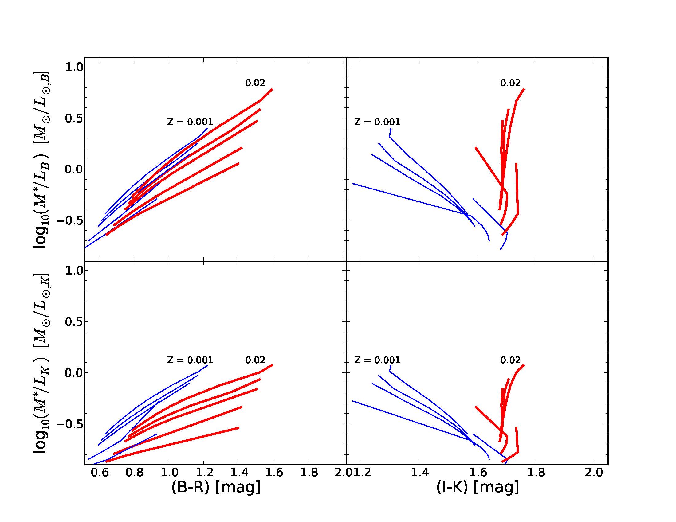 |
Figure 6. M* / L ratios for exponentially declining star formation rate models with different final age. The models are the same as in Figure 5, except that the populations are now observed 12, 8.5, 6, 3, 2 Gyr (top-to-bottom) after star formation commenced. The top ends of the lines are the ends with the smallest positive τ values, i.e. the oldest average age. For clarity, only the solar metallicity (Z = 0.02; thick red lines) and the 1/20th solar metallicity (Z = 0.001; thin blue lines) are plotted and the dashed lines connecting the same τ values are not shown as in Figure 5. In principle these models form similar grids with different offsets. Based on Maraston (2005) models. |
The main conclusion from the color-M* / L diagrams in Figure 6 is that a final age change mainly results in a simple offset since the slope of the relation stays nearly constant especially for solar metallicities. The age-metallicity degeneracy stays intact in the optical relations. Only at the youngest ages and lowest metallicities, and predominantly in M* / LK, does the slope of the relation change.
So far only smooth SFHs have been considered in this section, but star formation will be more bursty in nature for especially smaller systems. A recent burst of star formation will dramatically lower the M* / L of a total stellar system as well as change its SED to make it look much younger, because a young population is so much more luminous. The size of the effect will depend on the size of the star burst relative to the underlying population and the age difference between the populations. This effect may be most relevant for small galaxies, where any burst of stars is significant, and for stellar masses dominated by an old population, where any trickle of young stars will dramatically alter their properties. For instance, the rejuvenation caused by a "frosting" of young stars has been used to explain the apparent line indices based young ages of morphological ETGs that are thought to be mostly old (de Jong & Davies 1997; Trager et al. 2000), though hot horizontal branch stars produce the same effect on the observed line strengths (Maraston & Thomas 2000).
Figure 7 shows the effect of adding 10% of the final mass of the system in a star burst of 0.2 Gyr duration. The models start with the canonical set of 12 Gyr old exponential SFR models of Figure 5 to which 1, 2, 3, 4, or 6 Gyr old star bursts are added. For clarity, only the solar and 1/20 solar results are shown.
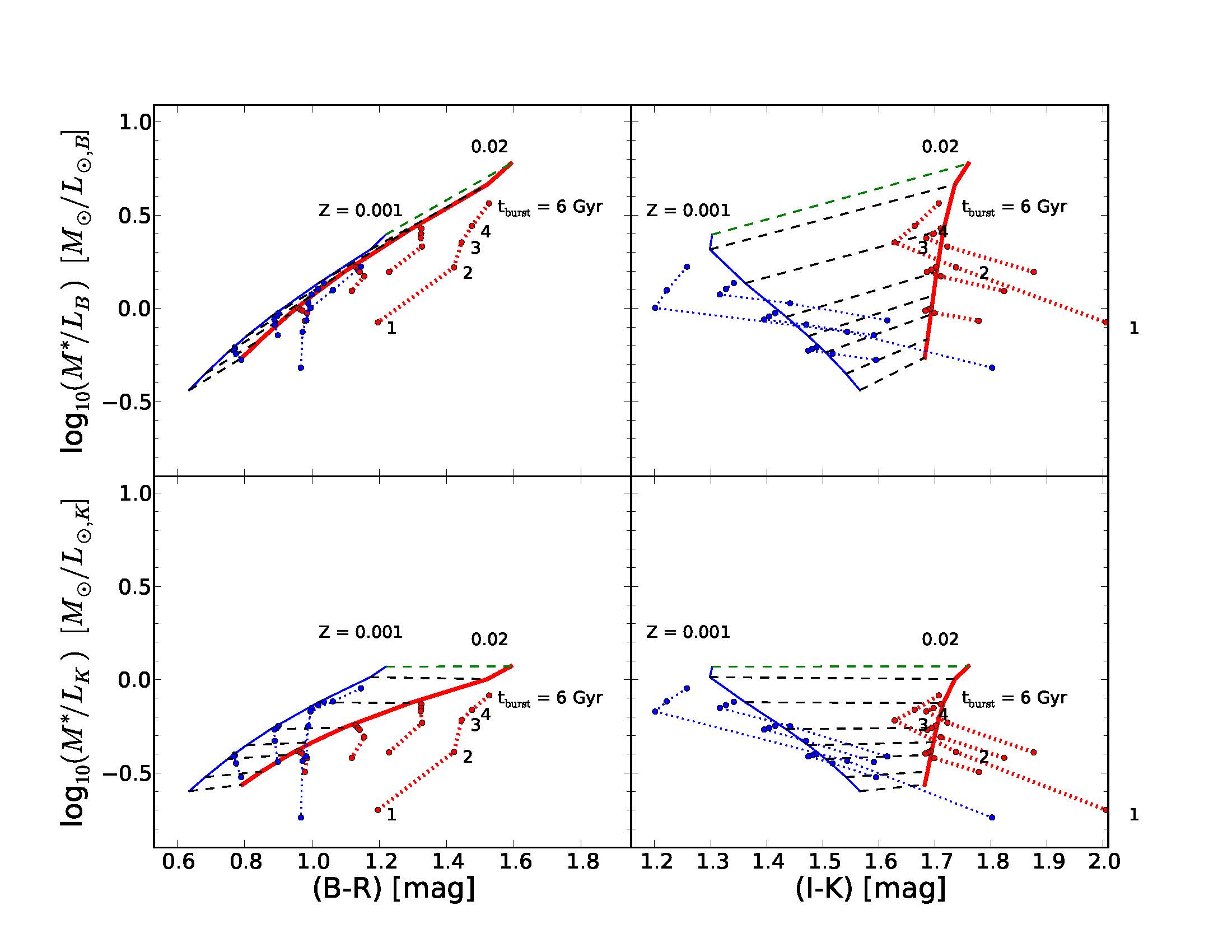 |
Figure 7.M* / L ratios for exponentially declining star formation rate models with an additional star burst. The starting models without starburst are the same 12 Gyr old exponentially decaying SFR models as in Figure 5, except that for clarity only the solar metallicity (Z = 0.02; thick red) and the 1/20 solar (Z = 0.001; thin blue) are plotted. For τ values ∞, 8, 4, 1 a 10% final mass fraction starburst of 0.2 Gyr duration is added that occurred 1, 2, 3, 4, 6 Gyr ago (solid circles connected with dotted lines). Based on Maraston (2005) models. |
A number of features are apparent from Figure 7. Firstly, the effects of starbursts are largest in both color and M* / L when starting with an a old, small τ population (independent of metallicity). Secondly, almost any burst of star formation will bias models towards lower M* / L values at a given color compared to smooth star formation models. At a given (B-R) color, the maximum offset from a smooth SFH due to a late starburst is less than 0.5 dex, but in most combinations it is less than 0.3 dex. This effect is stronger for higher metallicities. Finally, when starting off from a fairly young underlying population (τ > 5 Gyr) the effects of a the modeled starbursts are only larger than 0.1 dex in M* / L for bursts younger than 1-2 Gyr. In this case the population may actually become redder than the underlying population in (B-R) after a few Gyr after the burst, because the starburst will increase the luminosity weighted average age of the total population. When starting from mostly old populations (τ < 5 Gyr), the effect of a starburst on the M* / L may be long-lived (4-6 Gyr).
If most galaxies had irregular star formation in their last 2-5 Gyr with variations in star formation rate of factors greater than two, most galaxies are expected to lie below the smooth exponential SFR model SED-M* / L relations. One can calculate this offset and increase in scatter by using models that include a varying amount of star formation and incorporate this in the derived SED-M* / L relations. Alternatively, one can reduce the scatter induced by these recent star burst by including an SED tracer of a stellar population younger than 2-3 Gyr when fitting the SED. One has to chose a tracer that is not degenerate in age and metallicity with the other SED tracers used. Some options include a (U-B) color or a higher order Balmer line. The combination of such recent star formation indicators and SED templates with an irregular SFR should yield a scatter reduction in M* / L by ~ 0.1 dex if many objects with irregular SFR are contained in the sample.
More bandpasses (at least four) can provide additional degeneracy lift. For example, in the Maraston models a very red (I-K) color only corresponds to the TP-AGB dominated ages of ~1 Gyr, which is more pronounced in a small tau-model. Most models behave similarly in the optical bands, while the NIR is driven by the treatment of evolved phases, for which there is a strong variance within existing models (see also Section 2.3.3).
2.3.2. Stellar Initial Mass Function
As noted in Section 2.1, the IMF is a major uncertainty in SP modelling and M* / L ratios are strongly dependent on it. The IMF of external galaxies is in principle unknown (though see Tortora et al. 2013), but most IMFs determined for the Milky Way in the Solar neighborhood show a very similar behavior, namely a turnover in their logarithmic slope at about 0.6 Solar mass. The exact details of this turnover in IMF slope around this mass scale are poorly constrained (see discussions in e.g. Scalo 1986; Kroupa 2001; Chabrier 2003), but critically determine the total mass of the system. Figure 8 visualises the solar metallicity M* / L versus color relation using different IMFs, specifically the same as in Figure 3. The predicted relations are clearly very similar in shape for exponential SFR models and the plausible Salpeter or Kroupa IMF (the Chabrier and Kroupa IMF's behave very similarly). These different IMFs result primarily in offsets in zero-point of the M* / L versus color relations. These offsets are independent of metallicity and nearly the same whether one measures M* / LB or M* / LK.
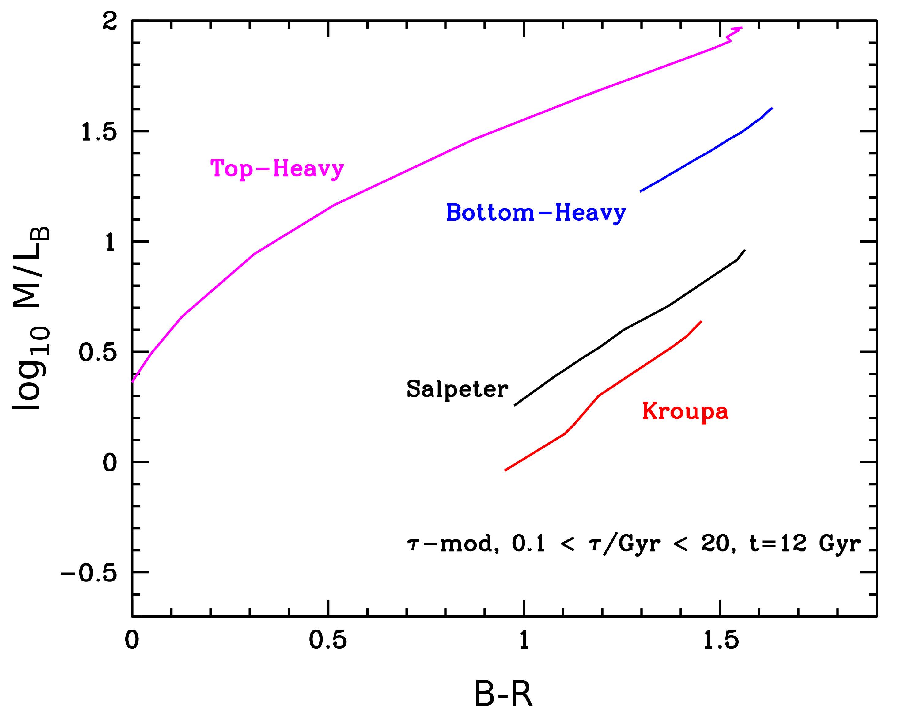 |
Figure 8. M* / L ratios vs (B-R) for exponentially declining star formation rate models of age 12 Gyr and solar metallicity, with a Salpeter, Kroupa and the same top-heavy and bottom-heavy IMFs as in Figure 3. |
The M* / L ratio versus color slope remains unchanged even assuming a rather extreme bottom-light IMF, but the offset is much larger (a factor of ~ 10) for the latter (Figure 8). However, this IMF is ruled out by strong gravitational lensing and stellar dynamics which only permit M* / L ratios up to a factor of ~ 2 higher than that predicted for a Salpeter IMF (e.g. Brewer et al. 2012; Cappellari et al. 2012).
As noticed in Section 2.1, EPS models include several ingredients and assumptions (stellar evolutionary tracks, stellar spectral libraries, IMF, etc.), which may be treated differently in different models. It is beyond the scope of this review to investigate the effects of each ingredient and its uncertainty on the models (for reviews see, e.g. Charlot et al. 1996; Maraston 2005; Conroy et al. 2009; Leitherer & Ekström 2012). Rather, M* / L versus color relations for the different EPS are compared here using exponential SFR models. The GALAXEV, PEGASE and FSPS models are used with a Chabrier IMF, while the Maraston models use a Kroupa IMF.
Not surprisingly, the GALAXEV (BC03) and PEGASE results are very similar in all color-M* / L diagrams, since they use the same Padova stellar evolutionary tracks and similar spectral libraries. At optical wavelengths, nearly all models agree to within 0.1 dex in (B-R) versus an M* / L measured in an optical band.
As discussed in Charlot et al. (1996) and Maraston (2005), the treatment of TP-AGB and RGB stars lead to the largest discrepancies in the NIR which is rehashed here with the (I-K) versus M* / L diagram. The (I-K) colors of old (small τ) populations with the same metallicity can differ by 0.2 mag, and up to 0.5 mag for young populations. The reason for this discrepancy is two-fold. Firstly, they are due to a different treatment of the (uncertain) late stages of stellar evolution (red supergiant, AGB, RGB). In these late stages, stars suffer mass loss that cannot be connected to the basic stellar parameters from first principles and must be parametrized and calibrated with data. This uncertainty involves energetics, stellar temperatures and stellar spectra for the AGB, and mostly stellar temperatures and spectra for the RGB. The importance of the TP-AGB phase of stellar evolution became clear, when it was shown that the BC03/Pegase/Starburst99 and Maraston (2005) models yielded systematic differences of several tenths of magnitudes in the NIR at intermediate ages of 0.2 to 2 Gyr (Maraston 2005; Maraston et al. 2006; Bruzual 2007), mostly attributable to differences in the treatment of TP-AGB stars. Secondly, numerical instabilities of luminosity integration along short-lived phases in the isochrone synthesis approach (see Maraston 1998; Maraston 2005) may explain why models based on the same stellar evolution tracks exhibit large fluctuations.
The models in Figure 9 with a small TP-AGB contribution (i.e. BC03, Pegase) display bluer values of (I-K) colors at young ages (low M* / L). The Vazdekis models would behave similarly, but they are redder only because they only include ages > 0.1 Gyr. Models with a substantial TP-AGB contribution Maraston (2005, GALEXEV 2007) display redder colors at young ages/large or negative τ's. At solar metallicity, old ages/small τ's (upper right corner of the diagram), models based on Padova tracks (B&C, FSPS, Pegase) are redder than the Maraston models based on the Cassisi et al. (1997) tracks because the former have a redder RGB (Fig. 9 in Maraston 2005, and discussion therein).
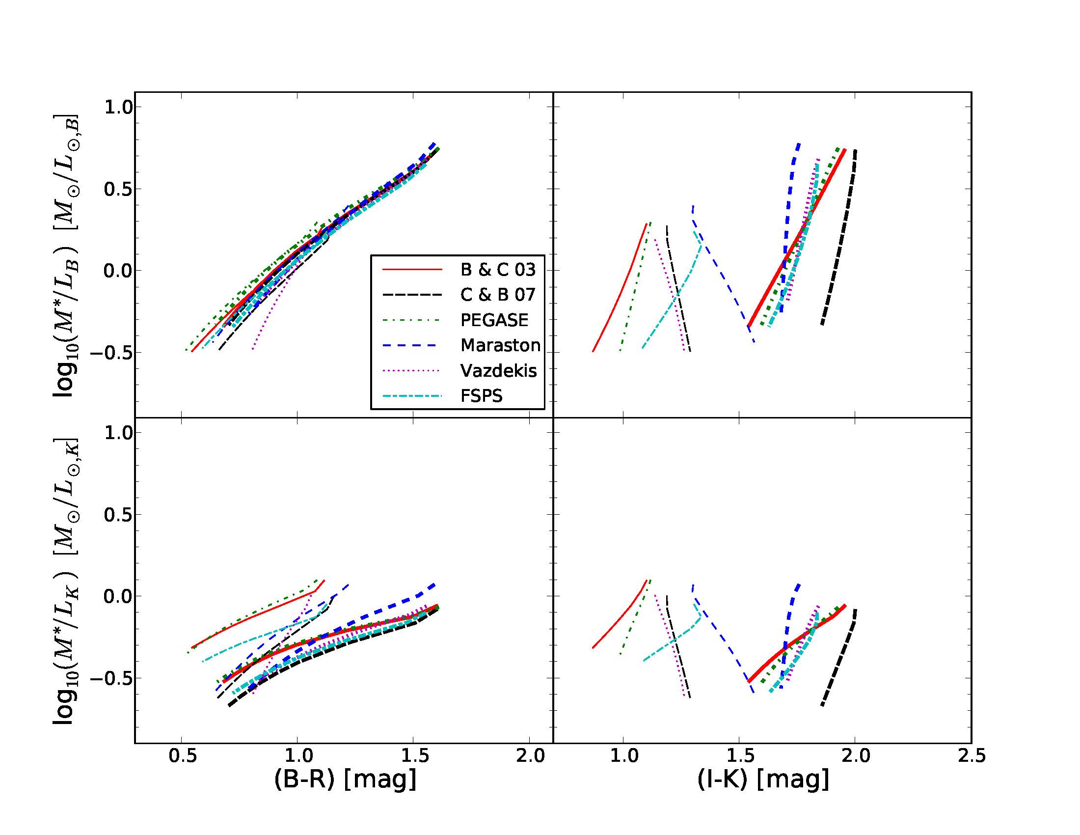 |
Figure 9. M* / L for exponential SFR models of age 12 Gyr using SSPs from different authors. The models compared are GALAXEV 2003 (Bruzual & Charlot 2003) with Padova 1994 tracks, GALEXEV (2007, an updated version of Bruzual & Charlot 2003 with different treatment of the TP-AGB phase), PEGASE 2.0 (Fioc & Rocca-Volmerange 1997), and the FSPS models (Conroy et al. 2009) all based on Padova stellar models and a Chabrier (2003) IMF, and the Maraston (2005) and the Vazdekis et al. (1996) models using a Kroupa (2001). Solar metallicity (Z = 0.02; thick lines) and 1/5 solar metallicity (Z = 0.004; thin lines) models are used, except for the Maraston models, where this metallicity is not available and a lower metallicity model of Z = 0.001 is plotted. The Chabrier and Kroupa IMFs give essentially the same results for broadband colors, hence by using these IMFs all the model sets can be compared even though some models are only available with either Chabrier or Kroupa IMFs. |
The variety of techniques to derive M* / L values by fitting spectra has increased dramatically in the last decade (e.g. Walcher et al. 2011). Methods depend on the data available, ranging from two bandpasses (e.g. Bell & de Jong 2001), multiple broadband colors (e.g. Bell et al. 2003; Maraston et al. 2012), a few line indices (e.g. Kauffmann et al. 2003; Thomas et al. 2011b) to full spectral fitting (e.g. Blanton & Roweis 2007; Tojeiro et al. 2009; Chen et al. 2012). Broadband imaging is often preferred over spectroscopy when large numbers of galaxies are required, when 2D stellar maps are created (Zibetti et al. 2009), or in low S/N situations as in high-redshift studies (e.g. Daddi et al. 2005; Shapley et al. 2005; Maraston et al. 2006; Cimatti et al. 2008). While more data points should in theory increase the accuracy of the M* / L estimation, this may not always be true in practice due to two reasons. Firstly, EPS models have larger systematic uncertainties at certain wavelengths (Figure 9). Such intrinsic model uncertainties should be taken into account while fitting the data, however this is rarely done (as it is not easy to quantify) and typically only the error in the measurement is used when weighing the different data points in the fit. Secondly, using more data points can also lead to systematic biases if the set of model templates is too limited to fit the complexity of the data. For example, long-ward K the SED is dominated by dust re-emission which is very difficult to model. Without a good description of dust re-emission, the fitting of far-IR data is meaningless and can even impede a proper understanding of shorter wavelength data. Another case is when smooth (e.g. exponentially declining) SFHs are used with data sets that include indicators very sensitive to recent star formation. In such cases, templates should include at least a combination of a smooth SFH and a late starburst.
Methods furthermore vary according to the number of templates fitted to the data, namely the range and type of SFHs and metallicity distributions (single burst, multiple burst, exponential SFH, etc.). This can lead to significant offsets whether one assumes that the most significant SF burst occured 12 Gyr ago (e.g. Bell & de Jong 2001) or more recently (e.g. Trager et al. 2000). Integrated light SEDs rarely contain enough information to discriminate between burst timescales 8-13 Gyr ago, which can lead to offsets as high as 0.2 dex in M*.
Finally, many mathematically different techniques have been used to fit models to data, ranging from simple minimum χ2 fitting (e.g. Bell et al. 2003), to maximum-likelihood (e.g. Kauffmann et al. 2003; Taylor et al. 2011), and Bayesian methods (e.g. Auger et al. 2009). For large data samples, information compression techniques are often used to reduce computational time, such as principle component analysis (Chen et al. 2012), non-negative matrix factorization (Blanton & Roweis 2007), and the linear compression technique used in MOPED (Panter et al. 2007). The optimum amount of reduction allowed while retaining all information available will depend on the data quality and model used and may be hard to determine (Tojeiro et al. 2007; Graff et al. 2011).
2.5. Robustness of Stellar Mass Derivations
Determining the accuracy and robustness of stellar mass estimation from SED fitting is non trivial since some of the intrinsic key properties of galaxies, most notably the SFH and the stellar IMF, are unknown. Nonetheless, estimates of uncertainties and systematic biases of a particular fitting method can be obtained by testing the results on mock galaxies. These mock galaxies are often based on semi-analytic galaxy formation models, providing hundreds of thousands of test galaxies with a wide range of (hopefully realistic) SFHs. Such comparisons can also provide guidance on the minimal and optimal data sets to use when fitting real data (Pforr et al. 2012; Wilkins et al. 2013).
The sections above make clear that several parameters affect the accuracy and biases of stellar mass estimates, the most important being: the IMF, data quality, EPS model, SFHs and chemical evolution, dust, and redshift. More detailed analyses can be found in, e.g. Conroy et al. (2009), Gallazzi & Bell (2009), Pforr et al. (2012), Wilkins et al. (2013), and references therein.
Firstly, the IMF is the main systematic uncertainty in M* / L estimation. However, as long as the IMF slope does not change for M > 1 M⊙, as is the case for Salpeter (1955), Kennicutt (1983), Kroupa (2001), or Chabrier (2003) IMFs, the incognita from the Initial Mass Function only results in a constant offset in stellar mass as the luminosity does not vary and only the total mass of a stellar population changes. A significant change of the IMF slope above M > 1 M⊙ implies a non constant offset (e.g. Pforr et al. 2012).
Constraints on the IMF normalization can be derived by comparing stellar population mass estimates to dynamical or lensing mass estimates such as described in the remainder of this review, with the simple notion that the mass in stars should not exceed the total measured one. Such a comparison is done in Bell & de Jong (e.g. 2001) using disk galaxy rotation curves. However, only upper limits can be obtained, since a fraction of the luminous mass can always be traded off to a (smooth) dark matter component with a similar mass distribution as the light. Only when there is a dynamical substructure on scales smaller than those expected for dark matter one can hope to obtain lower limits to the stellar mass normalizations. Examples include the dynamics of bar and spiral structure in disk galaxies, the effect of bulges on galaxy rotation curves, and the vertical velocity dispersion in disk galaxies (see Section 3). de Jong & Bell (2007) performed such a comparison between dynamical and stellar population mass estimates and showed that the SED-M* / L relation normalization can be constrained to within ~ 0.2 dex (66% confidence level). If the IMF varies amongst galaxy types, as argued for instance by Treu et al. (2010), Auger et al. (2010b), Cappellari et al. (2012) and Conroy & van Dokkum (2012) (see also Section 5.5.1 and Section 7.3.3), the IMF effect becomes much more complicated and unpredictable, let alone any evolution of the IMF with redshift (van Dokkum 2008).
Proceeding with random uncertainties, the accuracy of mass estimation depends on the quality of the data. For example, Gallazzi & Bell (2009) determine that a spectral signal-to-noise of S/N > 20 is required to get an accuracy of 0.1 dex in M* / L when using a few optical indices. Tojeiro et al. (2009) performing full spectral fitting derived a ~ 0.1 dex uncertainty in M* due to the quality of the data (S/N ~ 10-15 per pixel). Chen et al. (2012) exploited low S/N high-z spectra from the SDSS-III/BOSS survey to argue that spectral fitting relying on a principal component analysis can lead to reliable results also for S/N~5, though the actual parameters of the populations may not be well determined. Fitting the broad-band signal instead of the spectrum for the low S/N case may be the best choice (Maraston et al. 2012), and the two methods converge at high S/N.
The use of different EPS models also affects stellar masses, with an uncertainty of ~ 0.2 to 0.3 dex (on the logarithimic mass, Maraston et al. 2006; Conroy et al. 2009; Ilbert et al. 2010), reaching at most 0.6 dex at z ~ 2 (Conroy et al. 2009) when TP-AGB stars dominate the spectrum and the models vary most (see Section 2.3.3).
The adopted SFH in the models significantly contributes to the uncertainty and biases in M* / L values (e.g. Maraston et al. 2010) for high-redshift galaxies. The range in functional forms (if a function is used at all), the chosen oldest and youngest stars, and the inclusion and number of starbursts all affect the uncertainty and bias in the M* / L determination.
For galaxies at low-redshift with late star formation, Gallazzi & Bell (2009) find that the M* / L may be overestimated by 0.1 dex when using spectral indices. Nearly similar accuracies can be obtained using one optical color, the choice of which may vary with redshift (Wilkins et al. 2013). Using more than one color reduces the offsets slightly, but even more colors will not reduce the uncertainties and offsets (Gallazzi & Bell 2009; Zibetti et al. 2009). This is in apparent contrast with Pforr et al. (2012), who argue that more passbands further reduce uncertainties and stress the benefits of near-IR data. This may be related to the limited set of templates adopted by Pforr et al. compared to the star formation histories in their mock catalog (if the templates do not fully span the range of "observed" galaxy parameters, more data help getting closer to the correct result) and possibly due to their inclusion of dust effects. Pforr et al. (2012) also show that - when the template star formation history matches the real one - as is the case for positive tau models for high-redshift galaxies (Maraston et al. 2010), the mass recovery from spectral fit is excellent and mostly independent of the waveband used in the fit.
Indeed, from the point of view of the SFH, high-redshift galaxies have less uncertain M* / L as long as the redshifted data capture all necessary rest-frame wavelengths. This stems from a decrease in the number of possible SFHs (less time has passed since the initial star formation). Most notably the age difference between any old, underlying population and a recent burst is smaller, and the "frosting" or outshining effect by young stars is decreased (Maraston et al. 2010). For similar quality multi-passband data, this can reduce biases for dusty galaxies from 0.5 dex at z = 0.5 to 0.1 dex at z = 2 and uncertainties from 0.5 dex at z = 0.5 to 0.2 dex at z = 2 (Pforr et al. 2012).
Finally, dust in galaxies significantly alters the SED (e.g. MacArthur 2005). In case of very dusty systems spectroscopy clearly becomes the favoured channel for M* / L estimation. Access to both photometric and spectroscopic data would enable a derivation of extinction values by comparing SED expectations derived from the spectral features to the observed photometry (e.g. Kauffmann et al. 2003). Pforr et al. (2012) show that including dust prescription in the SED fit dramatically increases the uncertainties and biases in stellar M* / L estimates especially at low redshifts, with offsets being as large 0.5 dex and similarly sized rms uncertainties. When focussing on mass estimation, the conservative choice of neglecting dust as an additional parameter in the spectral fitting may lead to a more robust determination of stellar mass (Maraston et al. 2012).
The stellar mass of galaxies, M*, is a key parameter in studying the formation and evolution of galaxies over the cosmic time, tracing galaxy dynamics, and disentangling the contribution from dark matter to the overall galaxy potential. In this Section, we have reviewed the basic physics entering the derivation of M*. This exploits the theory of stellar evolution to calculate the mass in stars from the amount of stellar light that galaxies emit. The modelling of the integrated galaxy light requires several assumptions regarding the distribution of ages and chemical compositions of the component stars (i.e. the galaxy star formation history), the distribution of stellar masses at birth (the stellar initial mass function) and the attenuation of light from dust. The fundamental tool to perform such modelling is called a "Stellar Population model". We have described such models, highlighting their main uncertainties and how these affect the derivation of M*. Using models from various authors we visualised the basic relations between M* and the integrated spectral energy distribution, including color and spectral indices. Furthermore, we discussed the part of M* which is composed of stellar remnants, such as white dwarfs, neutron stars and black holes, which do not emit light but contribute to the total mass, and their dependence on the stellar initial mass function.
Finally, we briefly addressed the main techniques to calculate M* found in the literature and discussed the typical uncertainties and biases of SED based on stellar mass estimates. While these depend on galaxy type, they are: (i) for star-forming galaxies, the unknown star formation history and the fact that a small fraction by mass of newly born stars can outshine the underlying older population dominating the mass, thus jeopardising the mass derivation; and (ii) for both star-forming and passively evolving galaxies, the unknown IMF. Spectro-photometric data are most crucial for treating star-forming galaxies whereas the near-IR bands help in constraining the older, outshined component of the stellar population (see Figure 3 in Maraston et al. 2010).
Despite many unknowns, and excluding extreme cases of very dusty galaxies or galaxies with complicated and bursty star formation histories, relative stellar masses between galaxies can be regarded robust within 0.2-0.3 dex. The still poorly constraint IMF normalisation will shift SED derived M* / L values of all galaxies up or down by a few tenth of a dex, and if IMF variations occur across galaxy types and/or with redshift errors in SED, M* / L estimation may be as large as 0.5 dex. Recent simulations have shown how fundamental model parameters such as the choice of SFH, adopted wavelength range, redshift, and inclusion of dust, contribute to the uncertainties and can be used as a quantitative guide to assess uncertainties in M* (Maraston et al. 2010; Maraston et al. 2012; Pforr et al. 2012; Wilkins et al. 2013).
The most urgently required model improvements include constraining residual uncertainties in stellar evolution, specifically regarding the temperature of the RGB and the energetics of the TP-AGB stars, and the effect of non-solar abundance ratios on spectra. An improved understanding of star formation history effects for low-z galaxies would also be beneficial.
This review section is by no means complete, but it provides the necessary background to understand several statements made in forthcoming sections. Other comprehensive reviews which address stellar mass estimates in galaxies include Conroy et al. (2009), Greggio & Renzini (2011), Walcher et al. (2011), and Conroy (2013).
2 Note that bottom-light refers to an IMF that is not as rich in dwarf stars as the Salpeter one, namely has a different slope above 0.6 M⊙. This is different from a top-heavy IMF, which is strongly dominated by giant stars due to a smaller exponent value all over the mass range. Back.