


This section describes some of the basic bulk characteristics of distant dusty infrared star-forming galaxies. Included for discussion is the redshift distributions of DSFGs - how they have been measured in the past and how they will likely be measured en masse in the future - along with best estimates of luminosity functions and the total contribution of some DSFG populations to the cosmic infrared luminosity density or star formation rate density. Once redshift is in hand, we also discuss how one estimates the basic physical characteristics from a far-IR SED fit, whether using direct analytic fits or templates.
4.1. Acquiring Spectroscopic or Photometric Redshifts
Before the physical nature of individual DSFGs or the bulk nature of their population can be understood, redshifts are needed. As described in the first section of this review, § 2, redshift acquisition is unfortunately not straightforward for dusty, infrared-selected samples. Efforts to secure redshifts are hampered by significant extinction in the rest-frame ultraviolet and optical, where most of the classic emission-line redshift indicators lie, and the large beamsize of infrared/submillimeter observations which makes multi-wavelength counterpart identification ambiguous (see § 2.4.2).
The ambiguity of multi-wavelength counterpart matching has historically led to a dependence on intermediate bands for counterpart identification. § describes how radio wavelengths and mid-infrared 24 µm imaging has often been used as such an intermediate band by which counterpart galaxies can be identified on 1-2′′ scales, providing the precision needed to acquire redshifts.
In general, high-redshift galaxies may be studied in detail with either photometric or spectroscopic redshift identifications. Although the former is less precise and less reliable, the increase of available multi-wavelength coverage in deep extragalactic fields (e.g. as in the COSMOS field; Scoville et al., 2007) has made photometric redshifts increasingly reliable (e.g. Ilbert et al., 2009) and much less observationally expensive than obtaining spectroscopic redshifts. Spectroscopic redshifts for faint (i ~ 23 - 25) galaxies might require a few hours of integration on an > 8 m class telescope. One might conclude that, if no further analysis of the galaxies' optical/near-IR spectra are needed, photometric redshifts are preferable particularly when counterparts are ambiguous. However, there are a few important details which must be kept in mind when considering redshifts for DSFGs in contrast to more 'normal' high-redshift galaxies.
First, dusty, infrared-selected galaxies are subject to significant optical extinction. More than making counterpart identification difficult, this could impact the quality and reliability of photometric redshift estimates. Spectroscopic campaigns of ~ 500 M⊙ yr-1 850 µm-selected SMGs have often found bright emission lines with no detected continuum (Chapman et al., 2003b, 2005), with emission-line-to-continuum ratios far higher than observed in, e.g. ~ 10 M⊙ yr-1 Lyman-Break Galaxies (Shapley et al., 2003). The quality of photometric redshifts for SMGs, or any similar dusty, high-SFR DSFG, relies on the input stellar population model assumptions accounting for bursty star formation episodes, very significant extinction factors, and very high star formation rates. While a broad range of stellar population models have been successfully used to measure accurate photometric redshifts of optically-identified galaxies, no systematic study of their reliability for dustier, starbursts galaxies has been carried out, and often, photometric redshifts have been found to fail catastrophically for DSFGs (e.g. Casey et al., 2012b).
Second, in the era when submillimeter surveys had a smaller angular footprint on the sky, the preferred method of redshift acquisition was different. Pre-2009, the sky coverage of submillimeter maps was limited to a few square degrees scattered about the sky in a few legacy fields and around several galaxy clusters. The latter tended to lack sufficiently deep optical ancillary data needed to compute reliable photometric redshifts. Given individual areas only several-to-tens of square arcminutes in size, spectroscopic follow-up with instruments of a similar field-of-view was often more efficient and precise. Furthermore, spectroscopic identifications have the added benefit of facilitating follow-up kinematic and dynamical studies, like resolved Hα observations from adaptive optics IFUs or CO molecular gas observations 8.
Although more recent infrared observatories have dramatically increased the angular footprint of submm mapping, and thus dramatically increased the number of detected DSFGs, the same limitations in ancillary data apply, with most of the mapped sky not having sufficiently deep multi-wavelength data to analyze samples by photometric redshift or even secure reliable radio or mid-infrared counterparts for optical/near-infrared spectroscopic follow-up. For the most rare and scattered submillimeter sources on the sky, millimetric photometric redshifts might be the only initial handle we have on their redshifts, and perhaps millimetric spectroscopic redshifts are the most efficient follow-up technique. When considering different methods of redshift acquisition, the scale of survey, availability of ancillary data, and maximum science gain should all be considered.
4.1.1. Millimetric Spectroscopic Redshifts
While millimetric spectroscopic redshifts - the ability to spectroscopically confirm a DSFG directly in the millimeter via mm-wavelength molecular gas emission lines - were a pipe dream for much of the 2000s, the past few years have seen significant advances in the area. The primarily limitation in prior years was receiver bandwidth. Existing correlators' bandwidths were always too narrow to serve as an efficient method of searching for galaxies' redshifts. One of the first improvements in widening millimetric receivers' bandwidths came with WIDEX on the Plateau de Bure Interferometer (PdBI). WIDEX is a 3.6 GHz bandwidth dual polarization correlator, a factor of four improved over its predecessor correlators. In a few short years with a variety of widened receivers, this direct method of spectroscopic confirmation was proven, e.g. using the EMIR receivers at the IRAM 30 m (Weiss et al., 2009a), the Z-spec instrument at the Caltech Submillimeter Observatory (Bradford et al., 2009), Zeus also at the CSO (Nikola et al., 2003), the Zpectrometer on the Green Bank Telescope (Harris et al., 2007, 2010, 2012), the redshift search receiver for the the Large Millimeter Telescope (UMASS; Five College Radio Astronomy Observatory) or the upgraded receivers on the Combined Array for Research in Millimeter-wave Astronomy (CARMA, e.g. Riechers et al., 2010b). The benefits of the millimetric spectroscopic technique are huge: there is no uncertainty with respect to multi-wavelength counterpart identification and these galaxies are already detected in the millimeter and expected to have luminous mm emission lines facilitating spectroscopic identification. ALMA is optimally designed to follow-up DSFGs in the submillimeter and identify redshifts via, e.g., CO molecular gas or the Cii cooling line. This type of follow up has been done for brightly lensed DSFGs detected by the South Pole Telescope (Vieira et al., 2013). Figure 16 illustrates a composite millimeter spectrum from these blindly CO-identified DSFGs (Spilker et al., in preparation). Unfortunately this technique is not yet sufficiently efficient to obtain redshifts for substantially large populations of unlensed DSFGs (current limitations are to ≤ 100 for lensed DSFGs, and ≤ 10 for unlensed DSFGs), but once ALMA enters full-science observations, DSFG follow-up will become an efficient way of confirming source redshifts
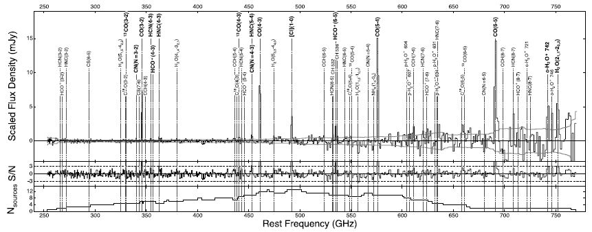 |
Figure 16. A composite, continuum-subtracted millimeter spectrum of 22 South Pole Telescope-detected brightly lensed DSFGs. These DSFGs constitute the most complete, unambiguously identified DSFG sample with spectroscopic redshifts. This figure is reproduced with permission from Spilker et al., submitted. |
4.1.2. Millimetric Photometric Redshifts
An alternate form of redshift determination which has gained some traction in the past few years is millimetric photometric redshifts (e.g. see Carilli & Yun, 1999, Hughes et al., 2002, Aretxaga et al., 2007, Chapin et al., 2009, Yun et al., 2012, Roseboom et al., 2012, Barger et al., 2012, Chen et al., 2013a). These 'millimetric redshifts' are determined from the shape of the far-infrared or submillimeter SED or its colors rather than any properties indicated by its stellar emission characteristics in the optical/near-IR or emission line signatures. This method assumes that the far-infrared SED of DSFGs is roughly fixed (e.g. to an Arp 220 SED, or an SED with some adopted representative temperature) and the FIR colors can be used to estimate the galaxy's redshift. This technique can be useful to roughly estimate sources' redshifts if they are impossible to probe using other methods.
An important observation to make about millimetric redshifts is that the precision can be quite poor and its accuracy is dependent on the intrinsic variation in SED types for the given population. As will be addressed in § 5.2, temperature, manifested as SED peak wavelength correlates with infrared luminosity and both can be degenerate with redshift. An SED which has a dust temperature between 30-50 K 9, the rest-frame peak wavelength can vary between 72-125 µm. If a 30 K SED is used to estimate that galaxy which peaks in the observed-frame at 400 µm, the millimetric photometric redshift will be z = 2.2. If the 50 K SED (approaching the temperature of some typical local ULIRGs, e.g. Arp 220 and Mrk 231) is assumed then the millimetric redshift will be z = 4.6. So while millimetric photometric redshifts can be quite useful to gauge the overall redshift regime of DSFGs (e.g. is it at z ~ 1 or z ~ 5?) and the bulk redshift distribution of a population, they should not be regarded as precise on a case-by-case basis. In contrast, several works use millimetric redshifts to study redshift distributions in a statistical sense, as in e.g. Greve et al. (2012), which can be useful to understand aggregate populations.
4.1.3. Redshift Distributions of 24 µm selected DSFG populations
Desai et al. (2008) and Fiolet et al. (2010) addresses the redshift distribution of 24 µm-selected sources by confirming a set of > 400 sources spectroscopically out of ~ 600 targeted. They find that the redshift distribution of 24 µm galaxies brighter than 300 µJy peaks at z ~ 0.3 with a possible second peak at z~ 0.9 and a tail of galaxies detected out to z ~ 4.5. This confirmed earlier photometric work on 24 µm sources in COSMOS (Le Floc'h et al., 2005) which finds the vast majority of sources at z < 1, with a clear link between 24 µm and K-band populations. Given the 24 µm observed selection function (shown in Figure 7), this is along the lines of what might be expected given the enhanced sensitivity of observed 24 µm at very low redshift and in certain redshift ranges that align the 24 µm band with bright PAH emission features (see more in § 5.7). Desai et al. (2008) also find a population of extremely infrared luminous DSFGs at z ~ 2 that, although difficult to spectroscopically confirm due to wavelength restrictions of optical spectrographs, were thought to be largely dominated by AGN-driven emission (~ 55%).
This population of z ~ 2 24 µm-selected DSFGs was studied in detail by Dey et al. (2008) who outline the selection of Dust Obscured Galaxies (DOGs) to especially target this extremely luminous subset of the 24 µm-population at ⟨ z⟩ = 1.99 ± 0.45. The AGN contribution to these DOGs' luminosity is estimated at ~ 50%, although this fraction is a function of observed 24 µm flux density, S24, with fainter targets less dominated by AGN-driven emission. Fiore et al. (2008) present a similarly selected population of galaxies as DOGs, although they approached the analysis using the fact that all of their targets were also AGN candidates. By stacking X-ray emission in the CDFS, Fiore et al. find that many of these DOG-like galaxies could harbor Compton-thick AGN. Read more about AGN content in DSFGs in § 5.6.
4.1.4. Redshift Distributions of 850 µm-1.4 mm-selected DSFG populations
The 850 µm-selected SMG population is the best-studied subset of DSFGs and their redshift distribution is illustrated in Figure 17. The initial assessment of the SMG redshift distribution came from Chapman et al. (2005), now one of the most well known compilations of DSFGs in the literature. Chapman et al. describe a population of 850 µm-selected SMGs which have radio counterparts; these radio counterparts have astrometric precision < 1′′ and provide excellent multi-slit spectroscopic targets. The Chapman et al. sample of 73 galaxies was spectroscopically observed at Keck Observatory using the LRIS instrument (Oke et al., 1995) and has a median redshift of z = 2.2 (some of these redshifts had been reported in earlier works, e.g. Barger et al., 2000, Chapman et al., 2003b).
 |
Figure 17. The redshift distribution of 850 µm and 870 µm-selected SMGs from the literature. The Chapman et al. (2005) redshift distribution (background solid blue) is a collation of 73 850 µm-selected radio galaxy redshifts obtained spectroscopically with the LRIS instrument on Keck 1 also including data from Chapman et al., 2003b. This distribution suffers from a radio flux limit at high redshifts (gray striped area) and a spectroscopic desert between 1.2 < z < 1.9 (this particular range is specific to the LRIS instrument on Keck 1). Sources with z ≳ 2 are primarily identified via Lyα emission and sources at z ≲ 1.3 are identified via OII, OIII or Hα. An updated version of the Chapman et al. redshift distribution is shown as a dashed-blue line, including DEIMOS-observed radio SMGs from Banerji et al. (2011) specifically targeted to fill the redshift desert gap of LRIS, and a handful of high-z 850 µm-selected SMGs (Coppin et al., 2009, Daddi et al., 2009, Walter et al., 2012). Also over-plotted is the Lewis et al. (2005) and Chapman et al. (2003b) phenomenological model 850 µm SMG redshift distribution without radio flux selection (dark green dot dashed line). We also over-plot the Wardlow et al. (2011) redshift distribution for the LESS 870 µm sample in CDFS (red line filled histogram) and the update to that sample - courtesy of ALMA follow-up establishing unambiguous counterparts - from Simpson et al. (2013) in orange. The latter is plotted in equal-time redshift bins to account for duty cycle correction. These redshifts are photometric and do not require radio sub-selection as a prerequisite, so they do not suffer from redshift deserts at intermediate or high redshifts, although a significant fraction (57/126) do not have any redshift indicators, primarily because they are too optically faint to characterize. Their relative contribution to this plot is given by the large line-filled red square on the right. |
Presented as is, this distribution (Figure 17) has two significant selection effects: (1) a required sub-selection in radio 1.4 GHz continuum, and (2) a dearth of sources between 1.2 < z < 1.9, which corresponds to the LRIS spectroscopic redshift desert. The requirement of radio detection in the Chapman et al. sample selects against galaxies at the highest redshifts since those galaxies are very unlikely to be 1.4 GHz-detected, as can been surmised from radio's positive K-correction as seen in Figure 3. Thus, radio sub-selection has cut off the high-z tail of the 850 µm distribution (as indicated by the hashed gray area on Figure 17). This is confirmed by the phenomenological models of Chapman et al. (2003b) and Lewis et al. (2005) who surmise that there should be a missing population of SMGs at high-z not detected in the radio. Chapman et al. also describe how radio sub-selection can also select against very cold-dust SMGs, as they'll have much higher S850 / S1.4 ratios than typical SMGs.
The second selection effect in the Chapman et al. sample is the LRIS redshift desert which spans 1.2 < z < 1.9. This is the redshift range for which no bright emission lines would be present in a galaxy's LRIS spectrum. At lower redshifts, the rest-frame optical features of OII 3727Å, Hβ 4861Å, OIII 5007Å, and Hα6563Å would be readily available. At higher redshifts, Lyα 1216Å would be accessible. In the desert, OII has redshifted too far out of LRIS' spectroscopic coverage and Lyα is not redshifted enough to be detected; LRIS' coverage at the time spanned ≈3000-8000Å. It is important to note that different optical multi-object spectrographs have different redshift deserts if they have different spectroscopic coverage. For example, the DEIMOS spectrograph on Keck (Faber et al., 2003) has approximate maximum coverage 4500-9500Å in low resolution mode, which corresponds to a redshift desert of 1.6 < z < 3.2, making it not as ideal an instrument for follow-up of a population which peaks at z ~ 2. Note that since the Chapman et al. (2005) spectroscopic survey has been conducted, the red arm of the LRIS instrument has been upgraded so the coverage now runs ≈ 3000-10000Å, with only a small desert around z ≈ 1.7.
Various efforts to remedy the biases of the Chapman et al. sample have been made. Several high-z (z > 4) 850 µm-selected SMGs have now been spectroscopically confirmed, including GN20 at z = 4.055 (Daddi et al., 2009), LESS J033229.4-275619 at z = 4.76 (Coppin et al., 2009) and HDF 850.01 at z = 5.17 (Walter et al., 2012), confirming that SMGs exist at the earliest epochs in the Universe's history, ~ 1 Gyr after the Big Bang. Banerji et al. (2011) also work to fill in the LRIS spectroscopic desert with spectroscopic confirmations from DEIMOS in the neighborhood of z~ 1.5. These have lead to a more contiguous picture of the 850 µm redshift distribution.
Wardlow et al. (2011) presented an optical/near-infrared photometric analysis to the 870 µm Laboca-selected population; the advantage of the Wardlow et al. sample is the Laboca map of the ECDFS is remarkably uniform in noise properties and fairly large. The 126 SMGs analyzed in that work represent one of the first complete and relatively unbiased samples of 850/870 µm-selected SMG populations. Furthermore, radio (or 24 µm) detection was not a necessary requirement for analysis as the paper goes to great efforts to estimate the 'missing' sources' redshifts through statistical groupings of near-infrared samples. The Wardlow et al. redshift distribution, perhaps not surprisingly, lacks some of the clear sample biases of the Chapman et al. sample and happens to resemble the Lewis et al. model redshift distribution peaking at z~ 2.5. Although more recent follow-up of the Wardlow et al. sample indicate that some of the Laboca sources split into multiples in ALMA imaging (Karim et al., 2013, Hodge et al., 2013b), the re-analysis of the population's photometric redshifts with the high-resolution data (Simpson et al., 2013) find largely the same results. This sample remains the only representative sample of the 850/870 µm population which has been unequivocally identified interferometrically and analyzed without substantial follow-up bias. Note that most differences between perceived median redshifts of 850 µm samples is due to depth and area limits of the given surveys. Brighter sources tend to sit at higher redshifts (Pope et al., 2006, Koprowski et al., 2013).
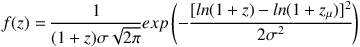
At slightly longer wavelengths, the AzTEC 1.1 mm-selected DSFG population has been studied in a little less detail than 850 µm-selected SMGs but provide equally large samples of ~ 100 galaxies with a good grasp on sample completeness. Figure 18 (left) illustrates the redshift distribution studies carried out at 1.1 mm. Beyond the millimeter photometric redshifts work by Aretxaga et al. (2007), Chapin et al. (2009) compile 28 secure redshift identifications for 1.1 mm-selected DSFGs in GOODS-N and measure a median redshift of z = 2.7 which they claim is statistically distinct from the z = 2.2 mean measured in the Chapman et al. sample and z = 2.5 in the Wardlow et al. sample. Yun et al. (2012) look at the 1.1 mm-detected DSFGs in GOODS-S and exploit the deep multi-wavelength ancillary data to measure redshifts as best as possible in the optical and near-infrared if spectroscopic redshifts do not already exist. Yun et al. also show that the millimetric redshift distribution of the sample is nearly identical to the optical/near-infrared redshift distribution, both of which have a median redshift of z = 2.6 ± 0.1, similar to the median redshift of z = 2.7 ± 0.2 found by Chapin et al. (2009). Yun et al. demonstrate that the 1.1 mm DSFG redshift distribution can be well-modeled by a log-normal distribution of the form
 |
(5) |
with zµ = 2.6 and σ = 0.2 in ln(1 + z). Although DSFG populations selected at other wavelengths do not often analyze the population with this parametrized fit, the shapes of most populations could largely be generalized in this form, with different mean redshifts and dispersions for populations selected at different rest-frame wavelengths.
 |
Figure 18. (Left:) The redshift distribution of 1.1 mm-selected DSFGs in the literature, all detected with the AzTEC instrument. The orange histogram represent secure redshifts (spectroscopic and millimeter photometric) from AzTEC sources in GOODS-N (Chapin et al., 2009) and the red is from AzTEC sources in COSMOS (Smolčić et al., 2012). The solid dark blue histogram represents both spectroscopic and optical photometric redshifts for AzTEC sources in GOODS-S (Yun et al., 2012) who suggest the distribution is a log-normal in nature with median value z = 2.6 (solid green line). The distribution in infrared photometric redshifts for the same GOODS-S sample is illustrated in hashed light blue to demonstrate its overall consistency with the optical spectroscopic/photometric sample. (Right:) The redshift distribution of 1.4 mm-selected DSFGs detected with the South Pole Telescope (Vieira et al., 2013, Weiss et al., 2013). The redshifts are all spectroscopically confirmed in the millimeter. The sample is known to be gravitationally lensed due to observing depth of observations and confirmed Einstein rings around many sources (Vieira et al., 2013), and since they are lensed, no sources are detected at z < 1.5. The mean redshift of the sample is z = 3.5, seemingly much higher than the mean redshift for 850 µm-selected or 1.1 mm-selected samples. |
One more notable analysis of the 1.1 mm-selected population is summarized by Smolčić et al. (2012) who describe interferometric follow-up observations of DSFGs in the COSMOS field. Like the interferometric work on the Laboca CDFS sample from ALMA (summarized in Karim et al., 2013, Hodge et al., 2013b), the Smolčić et al. work measures the accuracy of previous counterpart identifications to bolometer-detected sources and identifies submillimeter multiples (see more in § 2.5). Smolčić et al. suggest a revised strategy for assessing the optical/near-IR photometric redshifts of DSFGs by considering multiple minima in the χ2 photometric redshift fitting. They find a median redshift of z = 3.1 ± 0.3 for the 1.1 mm sample which is offset from the Chapin et al. and Yun et al. findings, but is also a small sample, consisting of only 17 galaxies. The discrepancy is most certainly due to the different strategy in analyzing photometric redshifts (including lower limits and choosing higher-redshift phot-z solutions) but it could also be due in part to cosmic variance, where the COSMOS field is known to have several notable, very distant DSFGs at z > 4.5 (e.g. Capak et al., 2008, Riechers et al., 2010b). At the moment, it is unclear to what extent the method of fitting photometric redshifts to DSFGs needs revision, as larger statistical samples are necessary to really determine the relative shortcomings of any redshift-distribution measurement technique.
Figure 18 (right) shows the observed FIR-spectroscopically-confirmed redshift distribution of 1.4 mm-selected DSFGs from Weiss et al. (2013). This sample is unique in that it consists of galaxies that are most certainly gravitationally lensed Vieira et al., 2013 because the 1.4 mm imaging from the South Pole Telescope is too shallow to detect distant DSFGs unlensed. Lensing does impact the observed redshift distribution since lower redshift galaxies (z < 2) are less likely to be gravitationally lensed by a foreground object than higher redshift galaxies. Weiss et al. (2013) argue that this effect is strong at z < 2, especially at z < 1, but it has little impact on lensing of higher redshift galaxies. In Figure 18 this lensing-bias is indicated by hashed gray areas at z < 2. The 1.4 mm redshift distribution is compared to several literature models which employ a phenomenological approach (Béthermin et al., 2012b), hybrid cosmological hydrodynamic approach (Hayward et al., 2013a), and semi-analytic approach (Lacey et al., 2010, Benson, 2012). It is important to stress that, although the SPT sample is small, these galaxies are the most spectroscopically complete DSFG sample of any; 26 targets were blindly chosen, for which 23 millimetric spectroscopic redshifts were measured from ALMA (their composite millimeter spectrum is shown in Figure 16). The Weiss et al. (2013) work also includes an interesting discussion of size evolution and its potential impact on the observed redshift distribution. If the mean physical size of DSFGs evolves with redshift (i.e. they are more compact or extended at high-redshift) then this behavior can impact the redshift distribution due to the influence of size evolution on lensing (Hezaveh & Holder, 2011). The more compact the higher-redshift DSFGs, the more likely it is for them to be detected in the 1.4 mm survey of lensed DSFGs. If the intrinsic redshift distribution of 1.4 mm-selected DSFGs mirrors the intrinsic redshift distribution of the 850 µm-selected SMGs, then a fairly extreme size evolution is needed to reconcile observations.
4.1.5. Redshift Distributions of 250 µm-500 mm-selected DSFG populations
Moving from long wavelengths to shorter wavelengths, here we address the redshift distribution of galaxies selected at 250-500 µm. Unlike surveys conducted at 850 µm-1.1 mm, BLAST, H-ATLAS and HerMES (see § 2.3.2 for details) have imaged several hundred square degrees of sky in large surveys. The nature of the galaxies detected in these large surveys is going to be more varied due to the large dynamic range in luminosities than those found in smaller surveys.
On small angular scales (< 1 deg2), the population of DSFGs which are luminous at 250-500 µm (at ≳ 20 mJy) might be thought of as very similar to 850 µm or 1.1 mm galaxies. In one sense, this is a correct assumption, since most galaxies which are ~ 5 mJy at 850 µm will be ~ 30 mJy at ~ 500 µm if they sit at intermediate redshifts z < 4. However, some important details are lost in this interpretation. Although most 850 µm-selected galaxies might be detectable at 250-500 µm, not all 250-500 µm galaxies will be 850 µm detected either because they sit at different redshifts or have different SED characteristics (see the discussion of the temperature bias of SMGs in § 2.4, also particularly Figure 20 of Casey et al. 2012a); more importantly, a population's selection wavelength (within 250-500 µm) matters quite a bit to their implied redshift distribution as pointed out by Béthermin et al., 2012b as 250 µm populations will be very different from 500 µm populations, where the latter more closely resemble the canonical 850 µm-selected SMGs.
By observing the increasing median redshift of samples with longer wavelengths in the previous section, one also might assume that longer wavelength populations correspond to higher redshifts, and shorter wavelengths lower redshifts. Thus, the 250-500 µm redshift distribution would peak below z ~ 2. This interpretation is partially correct since the peak of the dust blackbody emission does shift towards longer wavelengths at higher redshifts. However, this assumption can be too simplistic when not accounting for sample biases, intrinsic SED variation, and survey detection limits in the different bands. For example, a wide-and-shallow survey at 500 µm might overlap completely with a wide-and-shallow survey at 1.4 mm, in that they might both be efficient at picking up the same lensed dusty galaxies at high-z, but perhaps the equivalent deep pencil-beam surveys at the same wavelengths, 500 µm and 1.4 mm, reveal two completely different, non-overlapping populations. Therefore, it becomes important to clearly define population selection before comparing and contrasting distributions.
Figure 19 shows some of these contrasting populations selected at 250-500 µm, for both deep pencil-beam surveys and wide-field shallow surveys for lensed DSFGs. Negrello et al. (2007) present some of the first predictive measurements for 250-500 µm-selected lensed populations by combining physical and phenomenological models. Negrello et al. predict a redshift distribution for S350 > 100 mJy galaxies peaking at z ≈ 2 (red line on Figure 19). In contrast, earlier predictive work by Lagache et al. (2005) addresses the overall redshift distribution for the underlying 350 µm population, which peaks at substantially lower redshift, z ≈ 1, with a long tail out to high redshifts. Another phenomenological approach described in Béthermin et al. (2011), working backwards from constrained luminosity functions to redshift distributions and number counts predicts a peak at very low redshifts with a secondary peak 10 at z ~ 2. Béthermin et al. (2012b) present yet another new approach which is strictly empirical using the observed evolution in the stellar mass function of star-forming galaxies and the observed infrared main sequence of galaxies (Rodighiero et al., 2011, Sargent et al., 2012); they use empirical templates from Magdis et al. (2012b) as a function of main-sequence status to predict number counts and also source redshift distributions.
 |
Figure 19. (Left:) Redshift distributions of 250-500 µm-selected DSFGs in the literature and comparisons to model 250-500 µm predictions. Histograms have been renormalized since sample sizes vary from ~ 70 to ~ 2000 galaxies. The Amblard et al. (2010) distribution (blue hashed region) is generated through statistical means by fitting millimetric redshifts to ~ 2000 H-ATLAS Herschel-Spire 350 µm-selected DSFGs. The Chapin et al. (2011) distribution (purple hashed region) includes various efforts to characterize the 69 BLAST 250-500 µm-selected DSFGs in ECDFS (including spectroscopic and photometric redshifts collated from Dunlop et al., 2010, Casey et al., 2011a). The Casey et al. (2012a) distribution (solid green region) (also including data from Casey et al., 2012b) is a collection of ~ 1600 Herschel-Spire 250-500 µm-selected DSFGs, half photometric, half spectroscopically confirmed. The model distributions for this population are phenomenological and are described in Lagache et al. (2005) (magenta line), Negrello et al. (2007) (red line), and Béthermin et al. (2011) (orange line). (Right:) Redshift distributions of 450 µm-selected galaxies in the literature, observed with the Scuba-2 instrument, and contrasted to predictions and measurements of similar 500 µm galaxies observed by Herschel. The 500 µm Herschel sample (gray circles) is from an analysis of stacked data based on 24 µm priors and is suggested to peak at z ~ 1.5 (Béthermin et al., 2012b). At 450 µm, there are three datasets summarized in Chen et al. (2013a) (orange line histogram), Casey et al. (2013) (teal filled histogram) and Roseboom et al. (2013) (blue hashed histogram). The Chen et al. redshifts are millimetric photometric redshifts while the Casey et al. and Roseboom et al. are optical/near-IR photometric redshifts from COSMOS. The latter two samples overlap although are drawn from two different datasets; the Casey et al. dataset is more shallow and wide while the Roseboom et al. dataset is deeper and smaller. Casey et al. measure a median redshift of z = 1.95 ± 0.19 while Roseboom et al. measure z = 1.4. |
The first data results of redshift distributions in this regime came from Amblard et al. (2010) who use Spire colors of H-ATLAS sources to constrain redshift based on a millimetric redshift identification technique. Amblard et al. (2010) generate SEDs at a variety of redshifts and Spire colors and then identify the color-color space where most Spire sources are located and what redshifts they are most likely associated with. They estimate a median redshift of z = 2.2 ± 0.6.
Two more recent samples use both spectroscopic and optical/near-IR photometric redshifts to determine the 250-500 µm redshift distribution. Chapin et al. (2011) characterize the 69 BLAST-detected ECDFS sources, finding a flat distribution between 0.5 < z < 3 with a strong peak at z ~ 0.3. Casey et al. (2012a, b) summarize the efforts of a large spectroscopic follow-up campaign for ≈ 1600 HerMES Spire-selected galaxies in multiple fields covering ~ 1 deg2, nearly 800 of which are spectroscopically confirmed in the optical. They find a median redshift of z = 1.1 with peak around z = 0.8 with a long tail out to z ≈ 5. The Chapin et al. and Casey samples are statistically consistent when removing the z ~ 0.3 peak in the BLAST sample which is thought to be an over-density in ECDFS caused by cosmic variance. Both of these datasets agree with the Lagache et al. (2005) model distribution, potentially the Béthermin et al. (2012b) model distribution if some different SED assumptions are used, but are statistically distinct from the Negrello et al. (2007) model prediction for lensed galaxies.
The disagreement between the Amblard et al. (2010) and Chapin et al. and Casey results is likely due to (a) the assumptions about SED shape of Spire galaxies made by Amblard et al. (whereby a different assumed temperature-luminosity relation could have given a lower redshift peak) or (b) biases in the optical redshift samples which exclude higher redshift galaxies for lack of 1.4 GHz or 24 µm counterparts. Whatever the case, it is clear that work on the redshift distributions of Herschel-selected galaxies has not yet reached maturity.
In contrast to the large scale work done with Herschel, some further strides have been made at 450 µm using the Scuba-2 instrument on smaller scales. This population has not been probed until very recently since the 450 µm bolometers on Scuba were very difficult to use due to difficult sky subtraction. Although Sharc-II on the CSO probed this wavelength regime at 350 µm, Sharc-II was never used for mapping blank-field sky to detect its own population. The unique advantage of 450 µm mapping with Scuba-2 is its superb spatial resolution, ~ 7′′, which is significantly better than the spatial resolution of Herschel at 500 µm, ~ 36′′. Figure 19 (right panel) plots the redshift distribution for galaxies selected at 450 µm from data described by Chen et al. (2013a), Casey et al. (2013), Geach et al. (2013) and Roseboom et al. (2013) and compares it to some statistical determinations of the redshift distribution for 500 µm-selected galaxies from Herschel (Béthermin et al., 2012b, a). The 12-galaxy Chen et al. sample redshifts are derived from the millimeter (S450 / S850 colors) and span 0 < z < 6 with a median of z = 2.3. The Casey et al. sample and Roseboom et al. sample (the latter of which is the same dataset analyzed in Geach et al., 2013) sit in an overlapping region of the COSMOS fields. The Roseboom et al. map is ~ 1/4 the size of the Casey et al. map although it is also 4 times deeper (an RMS of 1.2 mJy versus 4.1 mJy). The respective redshift distributions could be drawn from the same parent population despite the fact that the quoted median redshifts for the samples are dissimilar (z = 1.4 in Roseboom et al. and z = 1.95 ± 0.19 in Casey et al.). The differences could be caused by the different field depths, where the Casey work extends over larger areas and is able to detect rare high-z systems while the Roseboom work is more sensitive to fainter galaxies at z ~ 1 - 2.
4.2. Infrared SED Fitting for DSFGs
Spectral energy distribution (SED) fitting in the far-infrared is needed to extract basic properties of galaxies' dust emission: its infrared luminosity, thus obscured star formation rate, dust temperature and dust mass. Far-IR SED fitting varies from the use of template libraries, the use of scaling relations, to direct data fitting to parametrized fits. Unlike data in the optical or near-infrared (Bolzonella et al., 2000, Bruzual & Charlot, 2003, Maraston, 2005), far-infrared data often suffers from a dearth of photometric data with far fewer bands available for comparison with models. At most, individual galaxies will have ~ 10 photometric data points in the far-infrared, and more like 3-5 on average, versus 30+ bands in the optical. Unfortunately, the parameters needed to describe the far-infrared emission are no less complex than those in the optical/near-IR, including dust distribution, composition, dust grain type, orientation, galaxy structure, AGN heating, emissivity and optical depth. Below we describe the techniques commonly used in the literature to measure far-infrared SEDs' basic characteristics and summarize them in Table 2. As a sidenote to all infrared SED fitting for DSFGs, the effect of far-infrared emission lines from CO or Cii should be considered, as emission lines can contaminate broadband submm flux densities by up to 20-40% (Smail et al., 2011).
SED fitting techniques can be broken down into categories: (1) direct comparison to models (radiative transfer or empirical) using, for example, χ2 techniques, (2) comparison with model templates using Bayesian techniques, or (3) direct FIR fitting methods to simple modified blackbody-like functions. The first two are described in § 4.2.1 and the last in § 4.2.2. Different applications of data call for different types of SED modeling. While the last set of methods is the most computationally straightforward to apply to galaxies with fewer data points, it might be useful for the user to fit the stellar emission and dust emission simultaneously, therefore use some of the more sophisticated models based on stellar synthesis modeling, accurate attenuation curves and dust grain analysis.
| Radiative Transfer Models | |
| Grasil; Silva et al. (1998) | Stellar population synthesis model which accounts for dust obscuration from UV through the FIR; incorporates chemical evolution, gas fraction, metallicity, ages, relative fraction of star-forming molecular gas to diffuse gas, the effect of small grains and PAHs and compares to observations from ISO. Can be used to investigate SFR, IMF, and supernova rate in nearby starbursts and normal galaxies. |
| Dopita et al. (2005) | Stellar population synthesis from STARBURST99 combined with nebular line emission modeling, a dynamic evolution model of Hii regions and simplified synchrotron emissivity model. Constructed for solar-metallicity starbursts with duration ~ 100 Myr and checked for consistency using local starbursts. |
| Siebenmorgen & Krügel (2007) | 7000 templates; spherically symmetric radiative transfer model accounting for a variety of star formation rates, gas fractions, sizes or dust masses. No accounting for dust clumpiness or asymmetry, although they argue it is insignificant. |
| Empirical Templates | |
| Dale et al. (2001), Dale & Helou (2002) | 69 FIR phenomenological models (Dale et al., 2001) supplemented by FIR and submm data presented in Dale & Helou (2002). SEDs are generated assuming power-law distribution of dust mass over a range of ISM radiation fields and constrained with IRAS and ISOPHOT data for 69 normal nearby galaxies. Mid-IR spectral features taken from ISO |
| Chary & Elbaz (2001) | 105 templates; used basic Silva et al. (1998) models to reproduce SEDs for four local galaxies (Arp 220, NGC 6090, M 82, M 51, representing ULIRGs, LIRGs, starbursts and normal galaxies) and ISOCAM CVF 3-18 µm observations to determine mid-IR spectra and continuum strength. Interpolated between four SEDs and used Dale et al. (2001) templates to create a larger range of FIR spectral shapes. |
| Draine & Li (2007) | 69 templates, 25 consistent with the most IR-luminous; model focused on mid-IR emission by balancing size distribution of PAHs with small grains, starlight intensities, and the relative fraction of dust which is heated by starlight. Checked for consistency against Spitzer data. |
| Rieke et al. (2009) | 14 templates, based on IRS and ISO spectra of eleven local LIRGs and ULIRGs connected to modified blackbodies with temperatures 38-64 K (where temperature scales with luminosity). Resulting templates span 5 × 10⁹ - 1013 L⊙ , where most luminous sources have strongest silicate absorption. |
| Energy Balance Techniques | |
| Magphys; da Cunha et al. (2008) | Constrains UV-FIR SED empirically using an energy balance argument. Accounts for wide variety of star formation histories and adjustable input stellar synthesis template library (which by default uses those from Bruzual & Charlot, 2003); attenuation determined from mix of hot and cool dust grains and PAHs. |
| Cigale; Burgarella et al. (2005), Noll et al. (2009) | Combines stellar population models from Maraston (2005) with Calzetti et al. dust attenuation curves and far-infrared SEDs from Dale & Helou (2002) to fit UV-FIR SEDs for a variety of galaxies. |
| Direct FIR-only Methods | |
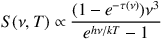
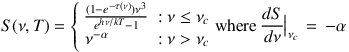
| Modified Blackbody | S(ν, T) = [(1 - e - τ(ν))ν3] / [ehν/kT - 1], where the optical depth is given by τ(ν) = (ν / ν0)β. β = 1.5 is a common assumption, although some work find its value varies from β ≈ 1 - 2. Most data indicates ν0 ≈ 1.5 THz. The optically thin assumption reduces the (1 - e - τ(ν)) term to νβ. |
| Two-temperature Modified Blackbody (e.g. Dunne & Eales, 2001) | S(ν, Tcold) + S(ν, Twarm),i.e. the sum of two modified blackbodies as given above. Tcold is here intended to dominate the FIR SED longward of ~ 100 µm, while the Twarm component helps reconstruct the emission at mid-infrared wavelengths. This procedure has more free parameters than the fitting methods below, so use with caution. |
| Piecewise Modified Blackbody+ Powerlaw (e.g. Younger et al., 2007) | S(ν,T) = {(1 - e -
τ(ν))ν3
ehν/kT - 1
: ν ≤ νc
ν - α
: ν > νc where dS / dν|νc = - α. Procedurally, this fitting method is identical to the modified blackbody fit, where the Wien side is removed and replaced by mid-infrared power-law consistent with any mid-IR data available; in the absence of mid-IR data, a powerlaw slope of α=2 is consistent with starbursts and slightly more shallow, ~ 1.5, for starbursts with AGN (Blain et al., 2003, Casey, 2012, Koss et al., 2013). |
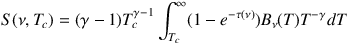
| Power-law of dust temperatures (e.g. Dale et al., 2001) | S(ν,Tc) = (γ - 1) Tcγ - 1 ∫ Tc∞ (1 - e - τ(ν)) Bν(T)T - γ dT , where Bν(T) is the Planck function and γ is a parameter determining the slope of the mid-IR power-law (note γ ≠ α). See Kovács et al. (2010) for fitting procedure. |
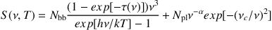
| Analytic Approx. Mod. Blackbody + Powerlaw (Casey, 2012) | S(ν,T) = Nbb(1 - e - τ(ν)) ν3 / ehν/kT - 1 + Npl ν - α e - (νc/ν)2 ; an analytic approximation to the power-law of dust temperatures fit which is computationally straightforward to fit to data. Npl is a fixed function of Nbb, the normalization factors, and νc is where dS / dν = - α, as is the case for the piecewise modified blackbody+ powerlaw fits. |
4.2.1. Employing dust radiative transfer models and empirical templates
Despite the relative lack of detailed data, detailed radiative transfer models and empirical template libraries have modeled the complex dust infrared emission from stars, molecular clouds and dust grains over a wide range of galaxy geometries and luminosities (Silva et al., 1998, Chary & Elbaz, 2001, Dale et al., 2001, Dale & Helou, 2002, Abel & Wandelt, 2002, Siebenmorgen & Krügel, 2007, Draine & Li, 2007). When discussing these models, it's important to keep in mind that the accuracy or applicability of these models cannot be tested with data since it simply does not exist in enough detail to disentangle effects of geometry, distribution, optical depth, etc. It's also important to note that many have done work in this area, particularly modeling radiative transfer in local starburst populations to generate SEDs (Efstathiou & Rowan-Robinson, 1995, Efstathiou et al., 2000, Efstathiou & Rowan-Robinson, 2003, Efstathiou & Siebenmorgen, 2009, Nenkova et al., 2002, Dullemond & van Bemmel, 2005, Piovan et al., 2006, Nenkova et al., 2008, Takagi et al., 2003, Fritz et al., 2006, Hönig et al., 2006, Schartmann et al., 2008), but here we try to focus on the techniques which have been most commonly employed for SED fitting of high-z dusty starbursts 11.
Silva et al. (1998) developed the Grasil code to model galaxy emission by explicitly accounting for dust absorption and emission from the ultraviolet through to the far-infrared. They use stellar population synthesis models and a chemical evolution code to generate integrated spectra for simple stellar populations of different ages, metallicities, star formation rates, gas fractions, relative gas trapped in molecular clouds versus diffuse ISM, dust geometry and dust grain size distribution (small grains versus PAHs). Chary & Elbaz (2001) use Grasil and the analysis of Silva et al. (1998) to generate template SEDs for infrared-luminous galaxies out to moderately high redshifts (z ~ 1) when measuring contributions of different galaxy populations to the CIB. Chary & Elbaz generate four SEDs with Grasil to fit data from nearby galaxies which each represent a different decade in infrared luminosity - Arp 220, NGC 6090, M 82, and M 51. They discard the mid-IR portion of the model spectrum and replace it with data from ISOCAM (Smith et al., 1989, Charmandaris et al., 1997, Laurent et al., 2000, Förster Schreiber et al., 2001, Roussel et al., 2001). They then interpolated between the four galaxies' SEDs to span intermediate luminosities. The templates were then split at 20 µm and additional FIR templates (20-1000 µm) were taken from Dale et al. (2001) to span a wider range of spectral shapes, i.e. dust temperatures.
In contrast to the Silva et al. (1998) and Chary & Elbaz (2001) work, Dale et al. (2001) present a different model for SEDs in the far-infrared. SEDs are constructed from various dust emission curves and the assumption that there is a power-law distributions of dust masses (thus dust temperatures) over a wide range of radiation fields. Small, large and PAH grains are all taken into account and the models are compared to data (from IRAS, ISOCAM and ISOPHOT) of 69 nearby normal galaxies for constraints. Dale et al. find that normal galaxy SEDs can be described solely by a range of FIR colors defined by the IRAS bands, i.e. S60 / S100. Dale & Helou (2002) builds on this phenomenological approach by extending calibration at wavelengths > 120 µm and correcting the Dale et al. (2001) model assumptions regarding dust emissivity and radiation field intensity.
Dopita et al. (2005) present another modeling technique which reproduces SEDs from the ultraviolet through the far-infrared, and out through the radio by combining stellar synthesis output from STARBURST99 (Leitherer & Heckman, 1995), nebular line emission modeling, a dynamic evolution model of Hii regions and a simplified synchrotron emissivity model to construct self-consistent SEDs for solar-metallicity starbursts with durations ~ 100 Myr. They describe the dependence of the far-infrared emission on the ambient pressure of the starburst. Although the Dopita et al. (2005) models are not often widely used amongst the high-z dusty galaxy community, their application could be appropriate, especially for solar-metallicity systems.
The Chary & Elbaz (2001) and Dale & Helou (2002) have garnered significant traction in the dusty galaxy community for SED fitting, particularly for galaxies detected in the mid-IR for which estimates of far-IR emission are necessary, but newer models have recently become available which make use of more sophisticated, later datasets and modeling techniques specifically tweaked for extreme starbursts.
Siebenmorgen & Krügel (2007) describe a spherically symmetric radiative transfer model for dusty starburst nuclei and ULIRGs and argue that the symmetry assumption, and lack of accounting for dust clumpiness, does not significantly change a dusty galaxy's SED. They present a library of 7000 SEDs which can be fit to galaxies either locally or at high-z and accurately be used to measure luminosity, size, dust or gas mass. Their SEDs have been applied in several more recent studies, e.g. Symeonidis et al. (2013), which study the bulk characteristics of FIR SEDs at high-z.
Draine & Li (2007) present another modeling method, focused instead on the emission from dust in the mid-infrared portion of the spectrum, but following through to the far-infrared. The models balance the size distribution of PAH grains and starlight intensities and the relative fraction of dust which is heated by starlight above a certain intensity. The models are constrained with data from Spitzer.
Another set of templates used extensively by the DSFG community are those described in Rieke et al. (2009). Rieke et al. use detailed Spitzer observations of eleven local LIRGs and ULIRGs to construct a library of templates spanning 0.4 µm-30 cm and luminosities 5 × 10⁹ - 1013 L⊙ . The spectral characteristics of the templates at rest-frame wavelengths ≲ 35 µm are comprised of IRS and ISO spectra, consistently matched to 0.4 µm - 5 µm stellar photospheric templates with a simple reddening law. The far-infrared portion of the spectrum is a modified blackbody with fitted temperatures ranging 38-64 K (70 < λpeak < 125 µm) and emissivity 0.7 < β < 1.
Contemporaneous to the works describing the latest empirical templates, Bayesian fitting codes have come about which are explicitly designed to fit observed data to template SEDs from the ultraviolet through the far-infrared. The Code Investigating GALaxy Emission (Cigale) was developed from an algorithm described in Burgarella et al. (2005) and formally presented in Noll et al. (2009). Cigale is based on model spectra generated in the optical/near-infrared by Maraston (2005) which account for thermally pulsating asymptotic giant branch (TP-AGB) stars, synthetic dust attenuation curves based on the modified laws presented in Calzetti et al. (1994) and Calzetti (2001) and far-infrared SED templates from Dale & Helou (2002). In contrast, the Multi-wavelength Analysis of Galaxy Physical Properties, or Magphys code, is a modeling package described in da Cunha et al. (2008) which empirically constrains the output of an SED from the ultraviolet through far-infrared using an energy balance argument. The infrared portion of SEDs are generated by modeling emission from hot grains (mid-infrared continuum; temperatures ~ 130-250 K), PAHs (mid-infrared spectral lines), and grains in thermal equilibrium (far-infrared continuum; temperatures ~ 30-60 K). The stellar component of SEDs is generated from Bruzual & Charlot (2003) stellar population synthesis, and the spectrum is attenuated using the angle-averaged model of Charlot & Fall (2000), and then the starlight which is attenuated in the optical is accounted for in the re-radiated infrared emission. The da Cunha et al. (2008) model technique is particularly versatile for constraining SEDs for galaxies of a wide range of star formation histories since any number of input stellar emission templates can be adjusted accordingly.
4.2.2. Direct modified blackbody SED modeling
In contrast to detailed models, many works instead approximate the far-infrared portion of the spectrum as a modified blackbody 12. Before the launch of Herschel, when DSFGs commonly only had one photometric point in the far-infrared - the photometric point corresponding to its detection band, e.g. 24 µm or 850 µm - even more simplistic interpretations of the modified blackbody were made simply because more sophisticated models would have been unconstrained. For example, in 850 µm-selected SMG samples, the 850 µm flux density was commonly converted directly to a far-infrared luminosity then star formation rate by assuming a modified blackbody of roughly fixed temperature, e.g. between 30-40 K, or an SED template of a local ULIRG like Arp 220 (Barger et al., 2012). The disadvantage of this method is that it does not account for variation in dust temperature which can impact the measured 850 µm flux density significantly for fixed infrared luminosity or star formation rate (see Figure 8 in § 2.4.1).
An alternate approach when only one far-infrared measurement is at hand is to use the FIR/radio scaling relation for starbursts (Helou et al., 1985, Condon, 1992, also see this review in §5.12). This empirical relation relates the rest-frame radio continuum luminosity of synchrotron radiation scattering off supernovae remnants to galaxies' rest-frame far-infrared dust modified blackbody emission and is shown to hold out to high redshifts in starbursts with either shallow or no evolution (Ivison et al., 2010a, b). With one far-infrared measurement and one radio continuum measurement, the integrated IR luminosity, thus star formation rate, is determined from the radio while the dust temperature of the modified blackbody is determined by the SED which best fits the given far-infrared data constraint. This was the procedure largely adopted for 850 µm-selected SMGs (e.g. Smail et al., 2002, Blain et al., 2002, Chapman et al., 2004a, 2005) and lead to the first measurements of SMGs' dust temperatures. The dust temperatures implied from the FIR/radio correlation were, as expected (Eales et al., 2000, Blain et al., 2004a, Chapman et al., 2004a), statistically colder on average than local ULIRGs by ~ 9 K, a difference which has been attributed to the dust temperature selection effect of 850 µm samples (Casey et al., 2009a, Chapman et al., 2010, Magdis et al., 2010).
DSFGs which do have more photometric constraints in the far-infrared, e.g. from Herschel Pacs and Spire bands (possibly in addition to other submillimeter data), a more sophisticated direct SED fitting can be done which does not rely on the radio luminosity or an assumed dust temperature. The most simplistic direct far-infrared SED fit is the blackbody fit, or Planck function, Bν(T) which is a function of temperature, T. However, given that galaxies' temperature is not uniform and inevitably variant, along with the fact that galaxies' dust is not perfectly non-reflective (source emissivity) and there is variation in opacity (i.e. non-uniform screen of dust), galaxies' flux density should be modeled as a modified blackbody of the form Sν ∝ (1 - e-τ(ν)) Bν(T), or
 |
(6) |
where S(ν, T) is the flux density at ν for a given temperature T in units of erg s-1 cm-2 Hz-1 or Jy. The optical depth is τ(ν) is defined by τ(ν) = κν Σdust and is commonly represented as τ(ν) = (ν / ν0)β, where β is the spectral emissivity index and ν0 is the frequency where optical depth equals unity (Draine, 2006), often assumed as = 3 THz from laboratory experiments (≈ 100 µm) although the measured value from a number of galaxies tends more towards 1.5 THz (≈ 200 µm Conley et al., 2011, Rangwala et al., 2011). The dust mass absorption coefficient has an identical frequency dependence, κν = κ0(ν / ν0)β, since τ ≡ κ Σdust. The spectral emissivity index, β, is often assumed to be 1.5 and is found to usually range between 1-2 in starburst galaxies (Hildebrand, 1983, Dunne & Eales, 2001, Chapin et al., 2011). Note that several works on nearby molecular clouds and dusty regions in nearby galaxies debate whether or not β also has temperature dependence, with laboratory experiments suggesting an anti-correlation (Lisenfeld et al., 2000, Dupac et al., 2003, Paradis et al., 2009, Shetty et al., 2009a, b, Veneziani et al., 2010, Bracco et al., 2011, Tabatabaei et al., 2013), although that has little impact on the implied SED fit for unresolved distant DSFGs where the effective temperature is only representative of the aggrigate dust temperatures contained within. Note that some works assume that DSFGs galaxies can be approximated as optically thin modified blackbodies, such that the (1 - e-τ(ν)) term reduces to νβ. This assumption is perfectly valid at long rest-frame wavelengths ≳ 450 µm where τ ≪ 1.
While the modeling of a single-temperature component modified blackbody goes a long way in accurately describing a galaxy's far-infrared emission, especially on the Rayleigh-Jeans tail of the distribution (where 850 µm-1.2 mm observations will sit), the short wavelength regime rarely provides a suitable solution. Most galaxies will exhibit a noticeable flux density excess at mid-infrared wavelengths above what is expected from the Wien tail, between ~ 8-50 µm rest-frame. This mid-infrared excess is generated from smaller clumps of hotter dust within the galaxy. Areas with more compact dust, particularly around a galaxy's nucleus, are more easily heated (either by star forming regions or AGN); higher energy radiation will more easily escape from an optically thin medium (see the thorough discussion of radial density distributions, dust clouds' opacity and dust mass coefficients in Scoville & Kwan, 1976).
There have been a few methods used in the literature to address the mid-infrared excess when fitting modified blackbodies. The first is to fit the SED to two modified blackbodies of different temperatures simultaneously. The cold component dominates the long-wavelength portion (corresponding to the vast cold dust reservoir), and a warmer component is used to make up the flux deficit at mid-infrared wavelengths. In fact, a number of works over the last decade have suggested using this two-component SED fitting technique (e.g. Dunne & Eales, 2001, Farrah et al., 2003, Galametz et al., 2012). Kirkpatrick et al., (2012) have argued that for a sample of high-z galaxies, a two component model may fare much better than a single component model. This said, this technique comes at the expense of introducing extra unconstrained parameters to fit (both dust temperatures, both normalizations, both emissivities).
Alternatively, other methods have dealt with this mid-infrared excess differently. First, several works fit the long-wavelength data (≳ 50 µm) to a single temperature modified blackbody and then cut-off the SED at short wavelengths and attach a power-law SED such that S(ν) ∝ ν-α where dS / dν ≲ - α (Blain et al., 2003, Younger et al., 2007, 2009b, Roseboom et al., 2013). In other words,
 |
(7) |
This is a very straightforward method which accounts for the mid-infrared excess, but has the disadvantage of not being easy to directly optimize simultaneously to a set of data which spans the divide at νc without first fitting the long-wavelength blackbody without the powerlaw. Another method is to assume instead that the aggregate SED is the composite of many SEDs of different temperatures, and the distribution of temperatures within a galaxy follows a powerlaw, such that
 |
(8) |
where the integrand is the modified blackbody from Equation 6 multiplied by T-γ, Tc is the critical or 'minimum' temperature which corresponds to the temperature of the most massive dust reservoir, and γ is a parameter of the fit which represents the slope of the powerlaw distribution in dust temperatures (see Kovács et al., 2010, for a detailed description of this method). This formulation is the most physically motivated method of fitting the mid-infrared portion of the SED through direct methods, but can be challenging to constrain as the integral must be computed numerically or can be alternatively written in closed form as an incomplete Riemann zeta function, Z(γ - 1, hν / kTc) and Γ(γ - 1) (see Kovács et al. for more). A fourth method for dealing with this mid-infrared spectral component seeks an analytical approximation to the power-law temperature distribution with
 |
(9) |
where the first component represents the long-wavelength modified blackbody and the second component represents the mid-infrared powerlaw (Casey, 2012). Here ν0 is the frequency where opacity is unity, α is the mid-infrared powerlaw slope, νc is the frequency at which dS / dν = - α and Nbb and Npl are the relative normalizations of the two components; Nbb is a free parameter and Npl is a fixed function 13 of T and β.
While much of the earlier work (2009 and prior) in direct SED fitting, particularly for 850 µm-selected SMGs, was based on the single temperature modified blackbody fit, more recent datasets, with coverage on both sides of the SED peak have lead to the latter fits, incorporating both cold-dust modified blackbody and mid-infrared powerlaw. All three methods will produce very similar fits with indistinguishable luminosities and peak SED wavelengths, although the choice of fitting method (e.g. least squares fit, generate templates and perform a χ2 test, etc.) can impact the subtleties of the fits (Kelly et al., 2012).
4.3. Estimating LIR, Tdust and Mdust from an SED
With an SED in hand, the measurement of infrared luminosity, LIR, is simply the integral under the curve in the infrared. The upper and lower limits of this integral are not completely standard in the literature, although most often are taken from 8-1000 µm (e.g. Kennicutt, 1998a). While 8-1000 µm is inclusive of all dusty emission, the drawback is that such a wide range captures multiple types of dust emission processes, from cold diffuse dust which dominates the long-wavelength portion of the SED to hot-dust and PAH emission in the mid-infrared (described more in § 5.7) to non-star formation driven heating, like AGN heating (§ 5.6). Non-star forming processes can come close to dominating the 8-1000 µm infrared luminosity, particularly for optically or X-ray identified AGN at rest-frame wavelengths ≲ 40 µm (Sanders et al., 1988, Koss et al., 2013). As a result, some works have pushed a narrower range of integration limits to restrict the computation of LIR to star-formation-driven emission only. This range is sometimes taken as 40-120 µm (from the IRAS-era, e.g. Helou et al., 1988) or a slightly broader range, 40-1000 µm. Despite the fact that these more restricted ranges carefully note that AGN could contaminate LIR(8 - 1000 µm by up to 25% for star-formation dominated DSFGs (and more for obvious AGN or quasars), the literature largely still uses the 8-1000 µm integration limits for historical reasons.
The conversion from LIR to star formation rate is not straightforward and relies on an understanding of the dust composition and initial mass function (IMF; see the review of Bastian et al., 2010). Most work on DSFGs assume the conversion given in Kennicutt (1998a) of
 |
(10) |
which takes the radiative transfer models of Leitherer & Heckman (1995) for continuous starbursts ranging in age from 10-100 Myr and a Salpeter IMF (Salpeter, 1955). Note importantly that this conversion does not account for AGN heating of dust in this wavelength regime, even though AGN fractional contribution is known to be non-negligible (10-30%). Here LIR corresponds to the full infrared 8-1000 µm; Kennicutt (1998a find that most other published work on calibrating this relation lies within ± 30%, notwithstanding differences based on IMF assumptions. Some more recent work (e.g. Swinbank et al., 2008) have assumed a Chabrier IMF (Chabrier, 2003) which alters the LIR to SFR calibration by a factor of ~ 1.8 or 0.23 dex, in other words, assuming a Chabrier IMF will produce star formation rates a factor of 1.8 lower than a Salpeter IMF. It is important to note that the conversion from LIR to SFR is only reliably calibrated locally for moderate-luminosity star forming galaxies. While high-redshift work in the literature have freely applied this scaling for lack of a better solution, it is not yet clear whether or not the conditions of this relation should change under different environments like more extreme luminosity systems at high redshift, and whether or not other dust-heating sources contribute significantly to infrared output, thus contaminating estimated star formation.
Besides LIR and SFR, a few other properties can be constrained from an SED fit including dust temperature, dust mass and emissivity index. As discussed in § 4.2.2, dust temperature scales with the inverse of the far-infrared SED peak, in other words, the wavelength at which the SED peaks in Sν, dubbed λpeak. However, critical to the interpretation of dust temperature, is the understanding that only λpeak is constrainable by current data and the conversion from λpeak, what is measured, to dust temperature requires a model assumption. Different assumptions in model dust opacity and emissivity can have dramatically different outcome dust temperatures, as shown in Figure 20. The differences generated by opacity assumptions (i.e. optically thin or ν0 value) dominate over emissivity assumptions (β value), although both can impact temperature measurements. Any work which hopes to compare temperatures between galaxies in the literature should have a firm understanding of the input model assumptions before interpreting differences, or rather, the comparison can be carried out in the observed quantity, λpeak.
 |
Figure 20. The relationship between SED peak wavelength, λpeak, and measured dust temperature, Tdust, for six different type of direct SED model assumptions. An unmodified blackbody SED, represented by the Planck function Bν(T) is shown in black and represents Wien's displacement law, i.e. λpeak T = b, where b ≈ 2.898 × 10 - 3 m K. The gray line is the relation for an optically thin modified blackbody as in Equation 6. Different assumptions regarding opacity, and under what wavelength regime it is equal to unity, are also shown, in green for the τ = 1 at 200 µm assumption and in blue for the τ = 1 at 100 µm assumption, with the darker shades denoting an assumed emissivity spectral index of β = 1.5 and lighter shades denoting β = 2.0. |
Both dust mass and emissivity spectral index are measured from the Rayleigh-Jeans regime of the infrared SED fit. In the optically thin regime (where Sν ≈ τ Bν(T)) dust mass is related to dust temperature and flux density via
 |
(11) |
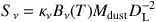
where κν is the dust mass absorption coefficient at frequency ν, Bν(T) is the Planck function at temperature T, Mdust is the total dust mass of the emitting body and DL is the luminosity distance. The modified blackbody is effectively represented by the product κνΣdust Bν(T), the product of a perfect blackbody, the dust mass coefficient and dust density. In this optical thin approximation, the galaxy's luminosity thus scales as Lν∝ Sν / Bν(T) ∝ ν-2. Note that at wavelengths shorter than rest-frame 350 µm, where the optically thin approximation breaks down, dust temperature has a profound effect on the dust mass measurement, since Bν(T) is highly dependent on T (Draine & Li, 2007); for example, a 4 K difference between 18 K and 22 K results in a 150% increase in measured Mdust. This dependence on dust temperature originates from the thermal emission per unit dust mass at a given λ being proportional to ∝(ehc/λ kT - 1)-1. Unfortunately the dust absorption coefficients are poorly constrained, particularly at short wavelengths, so the vast majority of dust mass measurements are taken at long wavelengths ~ 1 mm. Weingartner & Draine (2001) and Dunne et al. (2003) measure the dust absorption coefficient at rest-frame 850 µm to be κ850 = 0.15 m2 kg-1. A few corollaries from the dust mass calculation are the following proportionalities between dust mass, measured flux density, dust temperature, and infrared luminosity:
 |
(12) |
This highlights the fact that submillimeter flux density does not map simply to dust mass and that knowledge of the dust temperature, or λpeak, should be somewhat constrained. Note also that due to the lack of straightforward mapping of Sν to LIR, dust mass's relation to luminosity depends steeply on dust temperature. Dust mass can sometimes be used to derive gas mass via an assumed constant gas-to-dust ratio (e.g. Scoville, 2012, Eales et al., 2012, Scoville et al., 2013). Note however that this gas-to-dust ratio is only constrained in Milky Way molecular clouds and some local (U)LIRGs where molecular gas masses measured from millimeter lines can be directly compared to reliable dust masses measured from thermal continuum. A few high-z SMGs which have CO(1-0) observations (Ivison et al., 2011) have also been used to calibrate galaxies' gas-to-dust ratio ~ 100, which has been subsequently used to estimate some high-z DSFGs' gas masses (e.g. Swinbank et al., 2013.
It should be noted that there is a degeneracy between dust temperature and the emissivity spectral index β similar, yet not as pronounced as the degeneracy between dust temperature and assumed opacity model. Figure 20 illustrates this with different modified blackbodies using the same opacity models but with varying assumptions of β.
Coupling results from SED fitting and redshift acquisitions - giving you flux and distance - luminosity functions can be constructed. Unlike redshift distributions which extend out to z ~ 6 for DSFGs, infrared luminosity functions require additional understanding of sample selection and completeness so, as of yet, only extend to z ≈ 2 - 3. Luminosity functions studied beyond that redshift regime are very limited by sample selection effects, potential biasing and incompleteness. This subsection summarizes integrated luminosity function measurements made in the infrared for galaxies beyond the local samples detected by IRAS. We note that many works have also addressed the luminosity function in specific bands, e.g. 12 µm, 24 µm, 35 µm, etc., however these are not discussed here since they are less physical in nature than a discussion of the total integrated infrared luminosity, LIR (8 - 1000 µm) which should scale directly with infrared-based star formation rate.
The first measurements of the integrated infrared luminosity function out to z ~ 1 were carried out using Spitzer 24 µm data (Le Floc'h et al., 2005), extrapolating 24 µm flux densities to integrated infrared using local scalings and existing knowledge of mid-infrared spectral features and their impact on 24 µm flux with redshift. The 1/Vmax method of calculating a luminosity function uses the following methodology. The integrated luminosity function is given as
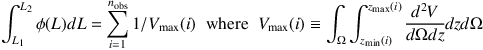 |
(13) |
where the the redshifts zmin(i) and zmax(i) define the maximum and minimum redshifts that source i would still have been accessible or detected in the given survey. While it presents the simpliest method of arriving at a volume density of sources, the 1/Vmax method might not be well suited for sources with increasing flux density at high-redshift (e.g. 1-2 mm detected sources Wall et al., 2008); however, alternative methods rely on model SED and redshift distribution assumptions. Further Spitzer work was presented in Caputi et al. (2007) and Magnelli et al. (2011), with similar conclusions as Le Floc'h et al. with the first extensions out to z ~ 2. Within uncertainty, results from the AKARI satellite out to z ~ 1.6 agree with Spitzer results (Goto et al., 2010).
Herschel-based luminosity functions have a clear advantage over previous Spitzer work since Herschel probes the peak of infrared emission directly rather than indirectly; work from Magnelli et al. (2009), Casey et al. (a, b), Magnelli et al. (2013b), and Gruppioni et al. (2013) have all published integrated luminosity functions all the way out to z ~ 3.6 using SED fits to PACS and SPIRE data. These Spitzer and Herschel luminosity functions are plotted together - segregated by redshift regime - in Figure 21.
 |
Figure 21. Measured integrated infrared luminosity functions from the literature, including work on the local RBGS sample (Sanders et al., 2003), Spitzer 24 µm-selected samples (Le Floc'h et al., 2005, Magnelli et al., 2009, 2011), and from Herschel via the PEP and HerMES surveys (Casey et al., 2012a, Magnelli et al., 2013b, Gruppioni et al., 2013). Here we only include data points themselves and not analytic approximations to the luminosity function, which is often given as a double power law. The four redshift bins are plotted with the same dynamic range, with the previous (lower) redshift bin illustrated in gray underneath to demonstrate evolution. |
Most literature presentations of the integrated luminosity function also present a analytic approximation, sometimes given as a Schechter function and sometimes as a double power law (Saunders et al., 1990). The double power law is represented as a function of four parameters (L⋆, Φ⋆, α, and σ) such that:
 |
(14) |
or, alternatively:
 |
(15) |
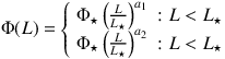
While all four parameters in Equations 14 and 15 are perhaps constrainable locally, no more than two can be constrained beyond z ≈ 0, so most works attempt to measure Φ⋆ and L⋆ by fixing α and σ (or in Equation 15, by fixing a1 and a2). Unfortunately, the uncertainties in the luminosity function itself mean that even 'fixed' parameters - α and σ or a1 and a2 - are themselves unconstrained, and fixing them arbitrarily results in different absolute calibrations of L⋆ and Φ⋆, as shown in Figure 22. Any physical interpretation of a measured L⋆ or Φ⋆ value should therefore be cautious. While the literature seems to uniformly observe an increase in L⋆ with redshift no matter which α and σ are assumed, despite absolute calibration off by ~ 1 dex, a concrete trend is not observed in the measured Φ⋆ values. It is critical to also recognize the interdependence of the two measurements; no abrupt 'break' or 'knee' is seen in the data, so a fit with high-L⋆ and low-Φ⋆ might be as equally adequate as a fit with low-L⋆ and high-Φ⋆. In the future, as more significant samples become available, Monte Carlo Markov Chains should be used to hone in on the key parameter values.
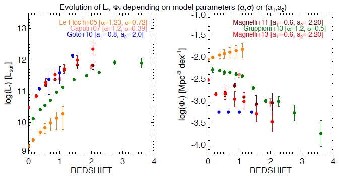 |
Figure 22. The evolution of L⋆ and Φ⋆ for the integrated infrared luminosity function from the literature. One of two models is adopted in these works. Le Floc'h et al. (2005), Caputi et al. (2007) and Gruppioni et al. (2013) all use the model described in Equation 14 while Goto et al. (2010), Magnelli et al. (2011) and Magnelli et al. (2013b) use the model from Equation 15. While L⋆ shows clear signs of downsizing in all models, irrespective of absolute calibration, the evolution in Φ⋆ is more model dependent. |
4.5. Contribution to Cosmic Star Formation Rate Density
The star formation rate density (SFRD) represents the total star formation occurring per unit time and volume at a given epoch; determining the contribution of infrared galaxies to the Universe's SFRD has been an important focus of DSFG surveys, particularly in understanding the role of dust obscuration at high redshifts. The SFRD is better constrained than infrared luminosity functions as the former is the integral of the latter. Like the calculation of the luminosity function, the 1 / Vmax method is most commonly used to form an understanding of a galaxy's accessible volume; in other words, given the limits of the survey (e.g. S850 > 2 mJy covering, e.g., 0.5 deg2), the maximum volume is found by shifting the given galaxy to higher redshift until that galaxy would no longer be detectable at its measured luminosity. The volume is then calculated based on that maximum redshift, and star formation rate is determined from infrared luminosity assuming a scaling like that of Equation 10. The infrared luminosity density (IRLD) may be calculated as an alternate to the SFRD, removing the uncertainty of the LIR - SFR calibration. As long as there is a clear understanding of a survey's depth and sky area coverage, the IRLD or SFRD is easily calculated as the total IR luminosity or star formation rate of the sample divided by its volume. Splitting the measurement into redshift bins then gives more detailed information on sample evolution. Plots of SFRD against redshift or look-back time are often referred to as a Lilly-Madau diagram, first discussed in Lilly et al. (1995) and Madau et al. (1996).
Figure 23 illustrates infrared-based estimates to the SFRD contribution from a variety of surveys and Figure 24 shows their contributions broken down by luminosity class. Both of these SFRD figures provide essential illustrations to the interpretation of cosmic star formation. While the first (Figure 23) includes samples known to suffer from incompleteness and biases, it is a useful tool for visualizing the net contribution from any one sample. For example, even though the 850 µm-selected SMG sample from Chapman et al. (2005) is known to be biased against warm-dust and radio-quiet galaxies, one can still determine that their SFRD contribution is ~ 10% of the total at z ~ 2. Knowing it is incomplete, one then knows that the real contribution is ≳ 10%. On the other hand, if the goal is to measure the total contribution of a population to cosmic star formation, then Figure 24 is more useful, as samples have been corrected for incompleteness and grouped in equal luminosity bins so as to compare like-with-like.
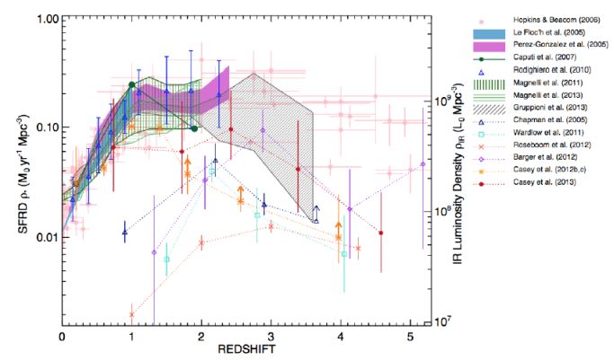 |
Figure 23. The contribution of various galaxy populations to the cosmic star formation rate density (left y-axis) or infrared luminosity density (right y-axis). The Kennicutt (1998a) scaling for LIR to SFR in Equation 10 is assumed. This SFRD plot shows the contributions from total surveyed infrared populations, whereas Figure 24 shows the break-down of contributions by luminosity bins between 0 < z < 2.5. All infrared-based estimates are compared to the optical/rest-frame UV estimates compiled in Hopkins & Beacom (2006) which have been corrected for dust extinction, and therefore represent an approximation to the total star formation rate density in the Universe at a given epoch. The total infrared estimates from the literature (integrated over ~ 108 - 1013.5 L⊙) come from Spitzer samples (Le Floc'h et al., 2005, Pérez-González et al., 2005, Caputi et al., 2007, Rodighiero et al., 2010, Magnelli et al., 2011) and Herschel samples (Gruppioni et al., 2013). In contrast, several samples from the submm and mm are also included; although they are known to be incomplete, they provide a benchmark lower limits for the true contributions from their respective populations. These estimates include 850/870 µm-selected SMGs (Chapman et al., 2005, Wardlow et al., 2011, Barger et al., 2012, Casey et al., 2013), 1.2 mm-selected MMGs (Roseboom et al., 2012), 250-500 µm-selected Herschel DSFGs (Casey et al., 2012a, b) and 450 µm Scuba-2-selected DSFGs (Casey et al., 2013). See legend for color and symbol details. |
As shown previously in, e.g., Le Floc'h et al. (2005), the contribution from ultraluminous infrared galaxies evolves strongly. ULIRGs have an insignificant role in cosmic star formation in the present-day Universe, but contributes ~ 10% at z ~ 1 and ~ 50% at z ≳ 2 (see Figure 24). The contribution from slightly less luminous galaxies - LIRGs - appears to peak at z ~ 1, as verified by multiple literature sources, amounting to ~ 50% of all star formation at that epoch. A key goal of the next several decades will be to improve the estimates of infrared samples' SFRD contributions out to higher redshifts with as much precision as the current optical and rest-frame ultraviolet estimates from pencil-beam surveys (e.g. Hopkins & Beacom, 2006) currently provide. Despite some limitations in infrared samples, the last decade's work on DSFGs has made it clear that dust-obscured star formation is non-negligible in the high-redshift Universe and should be studied carefully if one wishes to understand star formation processes at early times.
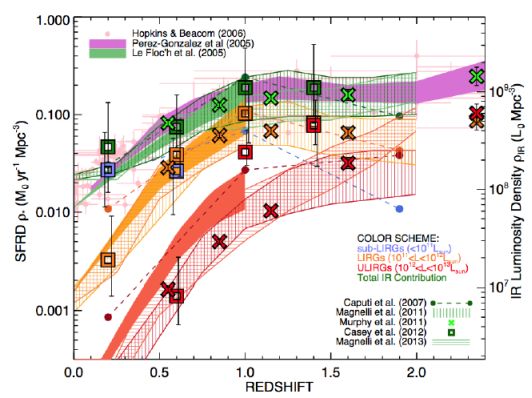 |
Figure 24. Estimates of DSFGs' contributions to cosmic star formation and infrared luminosity densities given by decade in luminosity. The overall color scheme adopted is that the total integrated infrared contribution is shown in green, the sub-LIRG population (i.e. L < 1011 L⊙) in blue, the LIRG population (1011 < L < 1012 L⊙) in yellow-orange, and the ULIRG population (1012 < L < 1013 L⊙) in red. The literature sources of each estimate are given by different symbols or line-types as indicated (Le Floc'h et al., 2005, Pérez-González et al., 2005, Hopkins & Beacom, 2006, Caputi et al., 2007, Magnelli et al., 2011, 2013b, Murphy et al., 2011, Casey, 2012). Note that not all literature derivations of different luminosity bins are computationally equivalent since some luminosities are derived directly from the far-infrared bands while others are extrapolations from mid-infrared bands. Most estimates agree within uncertainty in all luminosity bins, except the ULIRG estimates at z ~ 1, where Caputi et al. (2007) and Casey et al. (2012a) estimates are ~ 0.5 dex higher than those from Magnelli et al. (2011, 2013b) and Murphy et al. (2011). Overall, all datasets find the nearly insignificant role of ultraluminous galaxies at z ~ 0 while a dominating role of ultra-bright galaxies at high redshifts z ≳ 1.5. As more direct-FIR measurements become commonplace, the SFRD contributions from different luminosity types will be better constrained. |
8 Throughout the 2000s, the bandwidth for most millimeter line observations was narrow, so spectroscopic redshifts needed to be very secure to observe CO lines. Back.
9 Assuming a modified blackbody fit where the optical depth is unity at ~ 100 µm. Back.
10 This shape perhaps seems a bit counter-intuitive, but depends significantly on the input SED shape assumed for the population. Back.
11 While these models have been widely used to model the SEDs of high-z dusty starbursts, we do not recommend their blind use on large DSFG datasets without an intimate understanding of the governing parameters. Back.
12 Note that the term greybody is often used interchangeably with modified blackbody, however the former refers to the condition where the optical depth not wavelength dependent. Back.
13 When expressed in wavelength units, Npl = Nbb (1 - exp[ - (λ0 / λc)β])λc - 3 / exp[hc/λckT] - 1; see Casey (2012) for details. Back.