


This section describes the basic attributes of submillimeter/far-infrared maps and the scientific conclusions we can reach from direct measurement of those maps. While optical and near-infrared maps are fairly straightforward to interpret since there is a clear division between source and background, submillimeter maps from single-dish observatories are often dominated by confusion noise, where the beamsize is larger than the space between neighboring sources and it becomes difficult to pinpoint individual galaxies. Figure 10 illustrates the changing resolution over a single patch of sky in the COSMOS field from optical i-band through to 1.4 GHz radio continuum.
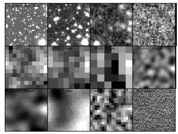 |
Figure 10. Twelve 1 × 1 arcmin cutouts from the COSMOS field imaged at different wavelengths with different facilities. From shortest wavelengths to long (top left to bottom right): Subaru i-band (0.8 µm), IRAC 3.6 µm, MIPS 24 µm, PACS 100 µm, SPIRE 250 µm, SPIRE 350 µm, SPIRE 500 µm, Scuba-2 450 µm, Scuba-2 850 µm, AzTEC 1.1 mm, MAMBO 1.2 mm, and VLA 20 cm (1.4 GHz). The resolutions vary substantially, from ~ 0.5′′ (i-band) to 36′′ (500 µm). This illustrates the challenge which most submillimeter mapping facilities in distinguishing individual galaxies which have a high spatial density. |
The community of submillimeter astronomers analyzing submillimeter maps have developed strategies to unravel the confusion brought on by large beamsizes; these techniques - including estimating positional accuracy, deboosted flux densities, sample completeness, etc - are described below in § 3.2. These techniques are essential to the analysis of large-beamsize submillimeter observations until more direct constraints (via interferometric observations) can be made. This review not only touches on the now-standard techniques for analyzing submillimeter maps, but also briefly describes different yet complimentary techniques, including stacking and a technique called P(D) analysis.
While the eventual goal of characterizing the sources in a submillimeter map is understanding the galaxies and their physical processes, this section describes a more basic measurement: submillimeter number counts. Number counts are simply the number of sources above a given flux density per unit area, often denoted N(> S) [deg - 2] in cumulative form or dN / dS [mJy-1 deg - 2] in differential form. Although the number counts might seem like a simple quantity to measure, inferring the number counts in the submillimeter can be challenging. The challenge is worth pursuing since number counts can provide key constraints on the cosmic infrared background (CIB), as well as galaxy formation theory (see § 10). Unlike studies of sources' redshifts, luminosities, SEDs, etc., the number counts measurement is not as plagued by sample incompleteness. Even without information on the physical characteristics of individual sources, number counts shed much needed light on the dominating sources of the extragalactic background light, EBL.
Confusion noise arises when the density of sources on the sky is quite high and the beamsize of observations is large; it is present when more than one source is present in a telescope beam. Optical observations are rarely confusion limited except in the case of very crowded star cluster fields, where the density of stars per resolution element is greater than one. However, confusion noise is far more common in the infrared and submillimeter given the large beamsizes of single-dish telescopes (see Table 1 in the previous chapter). Since fainter sources are far more numerous than bright sources, there will be some threshold in flux density beyond which a survey will become confusion limited. For a beamsize Ωbeam (an angular area), the confusion limit flux density Sconf is the limit at which the spatial density of sources at or above that flux density multiplied by the beamsize is unity. In terms of the cumulative number counts N(S) - the number of sources above flux density S - this confusion limit can be expressed where the following is fulfilled: Ωbeam N(Sconf) = 1. Even though an instrument or survey might be able to integrate longer to beat down instrumental noise, there will be minimal gain in field depth below the confusion limit.
3.2. Using Monte Carlo Simulations in Number Counts Analysis
The identification of individual point sources in a submillimeter map requires Monte Carlo simulations to characterize completeness, bias, and false positive rates. This technique was first outlined by Eales et al. (2000), Scott et al. (2002) and Cowie et al. (2002) and used in Borys et al. (2003) for the Scuba HDF survey and in Coppin et al. (2006) for the Scuba SHADES survey. It has since been updated for point source identification in Herschel extragalactic surveys such as HerMES (Smith et al., 2012), but probably the most elegant updates to the technique have come out of work done by the AzTEC team (see Perera et al., 2008, Scott et al., 2008, Austermann et al., 2010, Scott et al., 2012). These simulations go beyond the simple identification of sources; they provide a more accurate estimate of sources' intrinsic emission. By using a Markov Chain Monte Carlo statistical technique of analyzing submillimeter maps, sources' positional accuracy, intrinsic flux densities can be constrained, thus number counts, as well as sample contamination and completeness. The only major shortcoming of MCMC analysis is the lack of consideration of clustered sources, which might or might not be a significant effect (see § 7).
This technique is based on the injection of fake sources into noise maps. The distribution of sources in spatial density and flux densities, S, is an input assumption and the more the resulting source-injected map resembles the real data, the more accurate the input assumptions. The noise map used in these tests is often referred to as a 'jackknife' map and is constructed by taking two halves of the given submm data set and subtracting one from the other; then the noise is scaled down to represent the noise for the total integration time T (as a simple subtraction only represents an integration time of T/2). Since real sources should appear in each half of the data, they should not be present in the jackknife map, even at substantially low signal-to-noise. In that sense, the jackknife map represents pure noise.
With some assumption about the underlying distribution of sources in the field, individual delta function sources are convolved with the beam and injected into the jackknife map at random positions (assuming little to no influence from clustering) and, when finished injecting, the entire map is analyzed for source detections. If the distribution in individual point sources extracted from the resulting map mirrors the distribution of real data, then we have learned that the input assumptions might well be representative of the underlying parent population.
Determining an appropriate functional form of the input population (sources per unit flux density per unit sky area, dN / dS) is an iterative process, taking into account the functional form observed from the raw data map and the observed distributions at other submillimeter wavelengths. § 3.3 addresses the functional approximations of the differential number counts dN / dS. Whatever functional form is assumed, the free parameters of dN / dS are adjusted via a Markov Chain Monte Carlo until the differences between real and simulated map number counts are minimized.
Besides measuring agreement between real and simulated map number counts, a few other parameters can be estimated from the simulated maps. These include the positional accuracy of submillimeter sources, the difference between intrinsic flux density and measured flux density, and population contamination and completeness. Figure 11 illustrates an example flow chart of the simulations technique and the output estimates for the given dN / dS formulation.
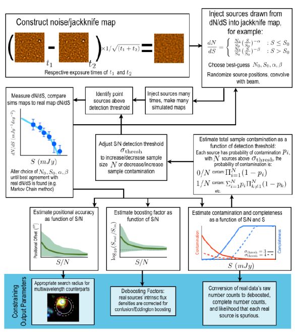 |
Figure 11. Flow chart illustrating the use of Monte Carlo simulations for analysis of submillimeter maps. The process begins with the construction of a jackknife or pure noise map in which real sources have been removed. Fake sources are then injected into the jackknife map using a number counts model assumption over several iterations. The parameters of the number counts can be optimized using a Markov Chain Monte Carlo technique. Once ideal parameters are determined, the positional accuracy, boosting factor of individual sources can be estimated, along with sample completeness and contamination. Analyzing the contaminating fraction within the whole sample can be used to determine the optimum detection threshold, σthresh. The final constraining output parameters of the Monte Carlo Simulations are: (a) the appropriate search radius to use when looking for multi-wavelength counterparts, (b) the deboosting factor to use when correcting a galaxy's raw measured flux density to intrinsic, and (c) how to convert raw number counts to incompleteness-corrected, deboosted number counts. |
3.2.1. Estimating Deboosted Flux Densities
One of the most critical output estimates from this technique is the correction for flux boosting. Sources' flux densities are boosted in two different ways. The first is the statistical variation around sources' true flux densities. More sources are intrinsically faint than bright, and therefore, more of those faint sources scatter towards higher flux densities than bright sources scatter down towards lower flux densities. This Eddington boosting (first described by Eddington, 1913) assumes that fainter sources are more numerous than brighter sources. The second form of boosting comes from confusion noise, as discussed in § 3.1, which is caused by sources below the detection threshold contributing flux to sources above the detection threshold. These two boosting factors are independent although their effect is the same so they are measured together as a function of signal-to-noise and flux density (both dependencies are important in the case where maps do not have uniform noise, see further discussion in Crawford et al., 2010). In simulations, the boosting is measured as an average multiplicative factor between input flux density and measured output flux density as a function of output signal-to-noise ratio. Boosting - or inversely, the deboosting factor - is estimated as a function of signal-to-noise because very high signal-to-noise sources are likely to only have a negligible contribution from statistical or confusion boosting.
Note that galaxies who benefit from gravitational lensing either will be detected at a substantially high signal-to-noise or substantially high flux density and thus, only be minimally affected by flux boosting. As the signal-to-noise of such sources becomes high, the fractional contribution of faint sources to measured flux density goes towards zero. Even in the case where the given submm survey is not substantially deep, sources with high flux densities well above the confusion noise threshold are unlikely to be substantially boosted as sources with comparable flux densities are exceedingly rare, and the only sources contributing to boosting will be negligible when compared to the instrumental noise uncertainty.
3.2.2. Estimating Positional Accuracy
Along with flux deboosting, the positional accuracy of submillimeter sources is estimated by contrasting the input 'injected' sources with the measured output sources. The output positions might be different from input positions due to confusion from sources nearby or instrumental noise. Like flux deboosting, positional accuracy is measured as a function of source signal-to-noise, as the sources of higher significance will only be marginally impacted by confusion. The average offset between input and output position is roughly indicative of the positional accuracy of submillimeter sources at the given signal-to-noise and has provided the initial search-area for corresponding counterparts at near-IR, mid-IR, and radio wavelengths (e.g. Weiss et al., 2009a, Biggs et al., 2011). Note, however, that Hodge et al. (2013b) use ALMA interferometric follow-up to determine that this method of determining positional accuracy is not completely reliable.
3.2.3. Estimating Sample Contamination & Completeness
Simulations also provide estimates for sample contamination and completeness and can guide a best-choice signal-to-noise (S/N) detection threshold. If a detection threshold is too conservative, contamination will be very low and completeness high, but the given submm source population risks being too small for substantial population analysis or more heavily biased against certain galaxy types, e.g. as 850 µm mapping biases against warm-dust systems, discussed in § 2.4.1. Conversely, a low detection threshold that is too liberal risks having a high contaminating fraction.
Sample completeness at a given flux density S can be estimated by considering the number of injected sources with S which are recovered in the simulated maps as real detections. The user can adjust the detection threshold to see increases or decreases in completeness. Note that nearly all submillimeter maps have non-uniform noise and that completeness is not only a function of flux density S but also detection signal-to-noise. Sample contamination is also measured as a function of output flux density and signal-to-noise as the fraction of detections which are not expected to be detected based on the input catalog. In other words, a source is considered a contaminant or spurious if the input flux density of sources within a beamsize is substantially lower than the nominal deboosted flux density limit. This can happen if the density of input sources with low flux densities is high, so the conglomerate of flux from multiple sources leads to a single 'spurious' source of much higher flux density. It can also happen when a single source of intrinsic flux density S is boosted significantly above the expected boosting factor at its signal-to-noise.
Together, the sample completeness and contamination can provide a good idea of what the strengths and weaknesses are of a given sample. These quantities can motivate the choice of a certain signal-to-noise threshold if there is a certain target contamination rate in mind. Often a target contamination rate of .5 ≲ 5% in a submillimeter map will result in a detection threshold between 3 < σ < 4. The contamination rate for an entire sample may be estimated using the probability that each individual source, of a given S/N, is real or a contaminant.
The measured number counts of a submillimeter map can be given in raw units - measured directly from the map - or deboosted and corrected units - after the sources' flux densities have been deboosted and the sample has been corrected for contamination and incompleteness. The latter is largely what has been published in the literature, albeit using slight variants on the method above used to correct the counts. Depending on the scale of the given survey (small, targeted deep field versus large sky area, shallow survey), the units of number counts are quoted direct or Euclidean-normalized units 7, given as galaxies per unit flux density per unit sky area (e.g. mJy-1 deg - 2 or Jy-1 str-1) and galaxies times flux density to the 1.5 power per unit sky area (e.g. mJy1.5 deg - 2 or Jy1.5 str-1, calculated as dN / dS × S2.5) respectively.
The 850 µm number counts are the best-studied amongst submillimeter maps with over 15 literature sources reporting independent measurements spanning four orders of magnitude in flux density; another regime where the number counts are fairly well constrained, although only recently, are at 450-500 µm, from recent Herschel and Scuba-2 measurements over three orders of magnitude. Figure 12 illustrates both 850-870 µm number counts (from Scuba, Laboca, Scuba-2, and ALMA Blain et al., 1999, Scott et al., 2002, Chapman et al., 2002, Cowie et al., 2002, Borys et al., 2003, Webb et al., 2003, Barnard et al., 2004, Coppin et al., 2006, Scott et al., 2006, Knudsen et al., 2008, Beelen et al., 2008, Weiss et al., 2009a, Karim et al., 2013, Casey et al., 2013, Chen et al., 2013a) and 450-500 µm (from Scuba, Herschel and Scuba-2 Smail et al., 2002, Oliver et al., 2010, Clements et al., 2010, Béthermin et al., 2012b, Geach et al., 2013, Casey et al., 2013, Chen et al., 2013a).
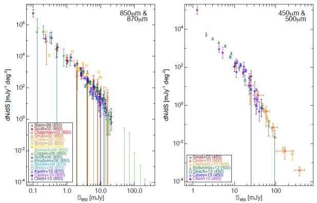 |
Figure 12. Differential submillimeter number counts at 850 µm/870 µm (left) and 450-500 µm (right). The 850 µm and 870 µm number counts come the initial Scuba surveys (Blain et al., 1999, Scott et al., 2002, Chapman et al., 2002, Cowie et al., 2002, Borys et al., 2003, Webb et al., 2003, Barnard et al., 2004, Coppin et al., 2006, Scott et al., 2006, Knudsen et al., 2008, shown in brown, dark red, red, dark orange, orange, dark gold yellow, light green, green, dark teal, and teal respectively). Data from Beelen et al. (2008), Weiss et al. (2009a), and Karim et al. (2013) are taken at 870 µm rather than 850 µm, the two former from Laboca and the latter from interferometric ALMA data. Scuba-2 850 µm data from Casey et al. (2013) and Chen et al. (2013b) are also plotted, the latter including the lens field work of Chen et al. (2013a). The Cowie et al. (2002) results do not quote uncertainties and the Barnard et al. (2004) results represent upper limits on number counts at very high flux densities, covering larger areas than the nominal Scuba survey. The work of Blain et al. (1999), Smail et al. (2002), Cowie et al. (2002), Knudsen et al. (2008) and Chen et al. (2013a) used gravitational lensing in cluster fields to survey flux densities < 1 mJy. |
Figure 13 illustrates other infrared and submillimeter number counts in the literature in direct units, from 70 µm (Dole et al., 2004, Béthermin et al., 2010a, Berta et al., 2011), 100 µm (Héraudeau et al., 2004, Rodighiero & Franceschini, 2004, Kawara et al., 2004, Berta et al., 2011, Magnelli et al., 2013b), 160 µm (Dole et al., 2004, Kawara et al., 2004, Béthermin et al., 2010a, Berta et al., 2011, Magnelli et al., 2013b), 250 µm and 350 µm (Patanchon et al., 2009, Oliver et al., 2010, Clements et al., 2010, Béthermin et al., 2010b, 2012), and 1.1 mm (Perera et al., 2008, Austermann et al., 2010, Scott et al., 2010, Hatsukade et al., 2011, Aretxaga et al., 2011, Scott et al., 2012).
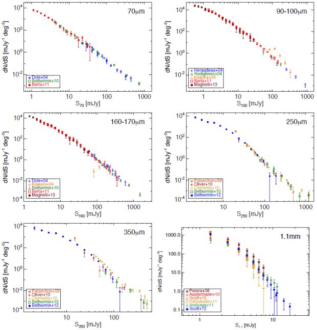 |
Figure 13. Differential submillimeter number counts at 70 µm, 100 µm, 160 µm, 250 µm, 350 µm, and 1.1 mm. The 70 µm data is collated from Spitzer MIPS (Dole et al., 2004, Béthermin et al., 2010a) and Herschel PACS (Berta et al., 2011). At 100 µm, data are from the ISOPHOT instrument aboard ISO (Héraudeau et al., 2004, Rodighiero & Franceschini, 2004, Kawara et al., 2004) and Herschel PACS (Berta et al., 2011, Magnelli et al., 2013b). At 160 µm-170 µm, data are from Spitzer MIPS (Dole et al., 2004, Béthermin et al., 2010a), ISO ISOPHOT (Kawara et al., 2004), and Herschel PACS (Berta et al., 2011, Magnelli et al., 2013b). At both 250 µm and 350 µm, data come from BLAST (Patanchon et al., 2009, Béthermin et al., 2010b) and Herschel SPIRE (Oliver et al., 2010, Clements et al., 2010, Béthermin et al., 2012b). All 1.1 mm number counts studies have been undertaken with the AzTEC instrument on JCMT and ASTE and summarized in Scott et al. (2012), including prior datasets described in Perera et al. (2008), Austermann et al. (2010), cott et al. (2010), Hatsukade et al. (2011), and Aretxaga et al. (2011). |
Figure 14 gathers all of these results together and plots all submillimeter number counts together in Euclidean-normalized units, allowing for a more clear view of how the slope, normalization, and intrinsic variance vary between selection wavelengths and what relative dynamic range is probed at each wavelength. § 3.6 goes into greater detail of what these measurements imply for resolving the cosmic infrared background.
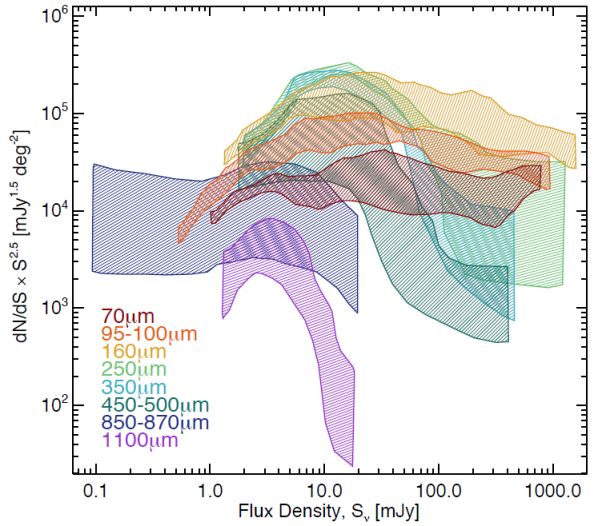 |
Figure 14. All differential submillimeter number counts replotted from Figures 12 and 13 in Euclidean units. For clarity in plotting, the individual points have been removed and replaced with a polygon representing the median 1σ spread in number counts measurements. |
3.4. Parametrizing Number Counts
Observed number counts are often fit to functional forms which assume a certain shape for the underlying distribution. This parametrization often is given as a Schechter function
 |
(3) |
or a double power law
 |
(4) |
While both typically provide reasonable fits to any given dataset over a narrow dynamic range, it is important to recognize that the shape of the number counts is probably intrinsically much more complex. Number counts represent flux density, not luminosity, so the conversion from a physically-motivated luminosity function to an observationally-derived number count function might not be straightforward. For example, if a Schechter function is the assumed shape to a luminosity function and that luminosity function evolves gradually with redshift, then the resulting number counts function will be non-Schechter; local galaxies influence the high flux density end, along with lensed galaxies, while the bump at lower flux densities is dominated by moderate to high-redshift galaxies (0.5 < z < 2.5, depending on the selection wavelength). An excellent paper summarizing power-law distributions in empirical data, their applicability and some common flaws in their overuse, is given by Clauset et al. (2007). The Clauset et al. discussion would be readily applicable to submillimeter number counts.
3.5. Bright-End Counts: Gravitationally Lensed DSFGs
Gravitationally lensed DSFGs constitute a significant fraction of the bright-end number counts at submm wavelengths at or above 500 µm. This is for two reasons. First, submm galaxy number counts are steep with a sharp intrinsic cut-off, thus flux magnification by gravitational lensing moves sources from the the steep faint end to the bright end and produce counts that are flatter at the bright flux densities (this was first discussed as an interesting sub-population in Blain, 1996). Second, due to negative K-correction, longer wavelength observations probe higher redshift galaxies where the optical depth to lensing is rapidly increasing (see Figure 6 of Weiss et al., 2013). At wavelengths shorter than 500 µm, while lensed DSFGs do exist, the bright-end counts are dominated by star-forming galaxies at low redshifts where the lensed counts do not make up an appreciable fraction (Negrello et al., 2007, Bussmann et al., 2013, Wardlow et al., 2013).
At all submm wavelengths the bright-end number counts can be reconstructed from local galaxies, active galactic nuclei such as radio blazars, and distant lensed infrared galaxies. The lensed sources can be identified relatively easily when submm maps are combined with multi-wavelength data. Local galaxies are easy to cross-identify through wide area shallow optical surveys such as SDSS while radio blazars are easily identifiable with shallow radio surveys such as NVSS. Theoretical predictions are such that at 500 µm, once accounting for local galaxies and radio blazars, lensed DSFGs should make up all of the remaining counts at S500 > 80 mJy (Negrello et al., 2007). This implies that there are no DSFGs at high redshifts with intrinsic 500 µm flux densities above 80 mJy. Observationally, this has yet to be properly tested but there are tentative results indicating that the lensed fraction is below 100% due to rare sources such as DSFG-DSFG mergers (Fu et al., 2013, Ivison et al., 2013). Existing followup results show that the sources that are neither associated with local galaxies nor radio blazars are gravitationally lensed with an efficiency better than 90% at 500 µm (Negrello et al., 2010, Wardlow et al., 2013). At 1.4 mm a similar (or better) success rate at identifying lensed DSFGs is clear with bright sources (S1.4 > 60 mJy) in the arcminute-scale cosmic microwave background (CMB) anisotropy maps made with the South Pole Telescope (SPT) (Vieira et al., 2010, 2013, ocanu et al., 2013). In Figure 15 at 1.4 mm from SPT in contrast to several models. In § 6 we will return to lensed DSFGs and review the key results that have been obtained with multi-wavelength followup programs. As the sources magnified, the improvement in both the flux density and the spatial resolution facilitates the followup of lensed galaxies over the intrinsic population.
 |
Figure 15. The 1.4 mm number counts of gravitationally lensed dusty sources from the South Pole Telescope from their 770 deg2 survey, after removal for nearby non-lensed IRAS-luminous galaxies. Three predictive models for unlensed and lensed galaxies are compared: Negrello et al. (2007), Béthermin et al. (2012b), and Cai et al. (2013). The Negrello et al. (2007) model combines a physical model from Granato et al. (2004) on the evolution of spheroidal galaxies with phenomenological models on starburst, radio and spiral galaxy populations. The Béthermin et al. (2012b) model is an empirical model based on two star formation modes - main sequence and starburst. The Cai et al. (2013) model is a physically forward model evolving spheroidal galaxies and AGN with a backwards evolution model for spiral type galaxies. This figure is reproduced from Mocanu et al. (2013) with permission from the authors and AAS. |
3.6. The Cosmic Infrared Background and P(D) Analysis
The total intensity of the cosmic infrared background (CIB) at submm wavelengths is now known from absolute photometry measurements (Puget et al., 1996, Fixsen et al., 1998, Dwek et al., 1998). While the integrated intensity is known, albeit highly uncertain, we still do not have a complete understanding of the sources responsible for the background, the key reason being that existing surveys are limited by large beamsizes and confusion noise. For example, recent deep surveys with Herschel and ground-based sub-mm and mm-wave instruments have only managed to directly resolve about 5% to 15% of the background to individual galaxies at wavelengths longer than 250 µm (Coppin et al., 2006, Scott et al., 2010, Oliver et al., 2010, Clements et al., 2010). At far-infrared wavelengths of 100 and 160 µm, deep surveys with Herschel/PACS have now resolved ~ 60% and 75% of the COBE/DIRBE CIB intensity (Berta et al., 2011). Additional aid from gravitational lensing in cluster fields and higher resolution 450 µm mapping with Scuba-2 mean that ~ 50% of the 450 µm background has been resolved (Chen et al., 2013a). The notable exception in this realm of direct detection of the faintest sources contributing to the CIB is the recent work of Hatsukade et al. (2013) who summarize the faint end of the 1.3 mm number counts from serendipitous detections within targeted ALMA follow-up observations. Assuming no correlation from clustering or lensing, they claim to resolve 80% of the CIB at 1.3 mm.
Note that Béthermin et al. (2012b) use a stacking analysis of 24 µm-emittors similar to the methodology outlined by Marsden et al., 2009, Pascale et al., 2009 using Herschel data to recover the FIRAS CIB and estimate the underlying redshift distribution of 250 µm, 350 µm, and 500 µm sources. The resulting estimates to number counts (extrapolated well beyond the nominal Herschel confusion limit) held up to more recent results from Scuba-2 (Chen et al., 2013a, Geach et al., 2013, Casey et al., 2013). Furthermore, Viero et al. (2013b) use a stacking analysis on ~ 80,000 K-band selected sources based on optical color selection, which is largely independent of mid-IR or far-IR emission. Viero et al. claim to resolve ~ 70% of the CIB at 24 µm, 80% at 70 µm, 60% at 100 µm, 80% at 160 µm and 250 µm, ~ 70% at 350 µm and 500 µm and 45% at 1100 µm. Of those resolved sources, 95% of sources are star-forming galaxies and 5% are quiescent. They go on to suggest that the galaxies which dominate the CIB have stellar masses ~ 109.5-11 M⊙ , and that the λ < 200 µm CIB is generated at z < 1 while the λ > 200 µm CIB is generated at 1 < z < 2.
While individual detections are confused by fainter sources, in maps where the confusion noise dominates over the instrumental noise, important statistical information on the fainter sources that make up the confusion can be extracted from the maps. Probability of deflection statistics, P(D) analysis, focuses on the pixel intensity histogram after masking out the extended (and sometimes bright) detected sources. The measured histogram in the data is then either compared to histograms made with mock simulation maps populated with fainter sources below the confusion with varying levels of number counts, both in terms of the number count slope and the overall normalization, or they are analyzed with the FFT formalism. With an accounting of the noise and noise correlations across the map, the simulations can be used to constrain the faint-end slope and count normalization that gives the best matching histogram to the data. Again, a major caveat of P(D) analysis is the lack of understanding for population clustering and its impact on residual flux in a map.
These P(D) statistics capture primarily the variance of the intensity in the map at the beam scale and, to a lesser extent, higher order cumulants of the intensity variation, again at the beam scale. P(D) method allows a constraint on the faint-end counts below confusion and has been used widely in sub-mm maps since the SCUBA surveys (Hughes et al., 1998). Patanchon et al. (2009) expanded the technique with a parameterized functional form for faint-end counts with knots and slopes. The number count model parameters extracted through the P(D) histogram data under such a model are correlated and these correlations need to be taken into account either when comparing faint-end P(D) counts to number count models or when using P(D) counts to distinguish cosmological models of the DSFG population. Extending below the nominal confusion limit of about 5-6 mJy of Herschel-Spire at 250-500 µm, P(D) studies have allowed the counts to be constrained down to the 1 mJy level. The parameterized model-fits to the P(D) counts resolve ~ 60% and 45% of the CIB intensity at 250 µm and 500 µm, respectively (Glenn et al., 2010). This is a significant improvement over the CIB fraction resolved by point sources counts alone that are at 15% and 6% at 250 µm and 500 µm respectively.
An alternative method, outlined by Refregier & Loeb (1997) involves the lensed intensity pattern through a massive galaxy cluster when compared to the intensity away from the cluster. The technique can be understood as follows: when viewed through the galaxy cluster, faint distant DSFGs will be magnified by a factor µ. But this resulting increase in the flux density is compensated by a decrease in the volume probed such that the total number counts seen through the cluster changes to N / µ. If the faint-end count slope scales as dN / dS ∝ S - α, then through the cluster is modified to dN′ / dS ∝ µα - 2 S - α. There is either an enhancement or a decrement of fainter sources towards the galaxy cluster, relative to the background population, depending on whether α < 2 or > 2. Averaged over the whole cluster, the effect will result in no signal as the total surface brightness is conserved under gravitational lensing. A measurement of the decrement has been reported with Herschel-Spire maps of four galaxy clusters in Zemcov et al. (2013). Instead of constraining the faint-end number counts below the confusion level authors used the lensing profile to obtain an independent measurement of the CIB level at Spire wavelengths, subject to uncertainties in the absolute flux calibration of Spire maps. They report a CIB intensity of 0.69-0.07+0.12 MJy sr-1 at 250 µm. The COBE CIB measurement at 240 µmis at the level of 0.9 ± 0.2 MJy sr-1 (Puget et al., 1996, Fixsen et al., 1998, Dwek et al., 1998). While the two agree within one σ uncertainties, the lensing-based measurement is likely an underestimate as it only focuses on the sources behind the cluster and a separate accounting of the sources in the foreground needs to be made to obtain the total background intensity. In any case the demonstration of Zemcov et al. (2013) shows that more detailed statistical measurements on the fainter source can be obtained through galaxy cluster lensing and the expectation is that future instruments, including ALMA, will exploit this avenue for further studies.
7 Euclidean-normalized units in this context are normal number counts multiplied by flux density to the 2.5 power. They are useful for converting an observed function which varies over several orders of magnitude to something relatively 'flat' where functional fits to data are performed simply and the extreme ends of the datasets do not dominate fit solutions. Back.