8. MOLECULAR GAS AND STAR FORMATION

This section reviews the status of both observations and theory of the star-forming molecular (H₂) gas in high-redshift DSFGs. When necessary, we provide some background into local observations to serve as a reference point. Other reviews in the last decade in this field can be found in Solomon & Vanden Bout (2005), Omont (2007) and Carilli & Walter (2013).

8.1. Basic Definitions

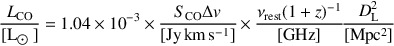
The amount of molecular line emission observed from a galaxy is typically expressed as the line luminosity. Here, we will take the example of CO as the emitting molecular line. CO could, in principle, be swapped out for other molecular species. The line luminosities are defined as either L_CO, or L′_CO. These are Solomon & Vanden Bout, 2005:

(18)

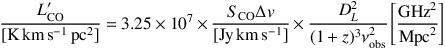
S_CO Δ v is the velocity integrated CO flux (Jy - km s^-1), ν_rest is the rest frequency in GHz, D_L is the luminosity distance in Mpc, and L_CO has units of L_⊙. L_CO is a measure of the total energy output from the CO line. Alternatively, the areal-integrated CO intensity L_CO^′ is defined as:

(19)

where the pre-factor 3.25 × 10⁷ is simply c² / 2k (scaled by powers of 10 to make the rest of the units comply), and k is Boltzmann's constant. L′_CO is typically used to convert from a CO luminosity to an H₂ gas mass (see the discussion in § 8.2).

Exciting a molecular line is done through a combination of collisional and radiative excitation. When lines are optically thick, line photon trapping can enhance molecular excitation. A convenient metric for thinking about the conditions necessary to drive the excitation of a given molecular line is the critical density. This is the density at which the Einstein A coefficients for spontaneous de-excitation out of a level is equivalent to the collisional excitation rate into a level: n_crit = A / γ. A summary of critical densities for a number of commonly observed molecular and atomic line transitions is given in Carilli & Walter (2013) for T = 100 K. Oftentimes it is assumed that if a line is observed, the densities present in the emitting gas are above the critical density for the line excitation. However, as pointed out by Evans (1999), this is too simplistic of a picture. In reality, a combination of collisional excitation and line pumping of excitation levels can be a significant enough effect that the effective density (n_eff ≈ n_crit / τ_line) for excitation can be much lower than the critical density. The effective densities to produce a 1 K line for a variety of molecules and transitions are given in Evans (1999) and Reiter et al. (2011).

8.2. Deriving H₂ Gas Masses from High-Redshift Galaxies

As one of the principle uncertainties in deriving molecular gas properties in galaxies at all redshifts is converting from the observable, carbon monoxide emission lines (hereafter, CO), to the physical quantity of interest, molecular hydrogen (H₂) gas mass, we briefly review what is known about the infamous CO-H₂ conversion factor. We note that an excellent in depth review of the topic has recently been written by Bolatto et al. (2013).

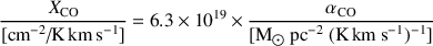
The CO-H₂ conversion factor is alternatively monikered X_CO (or the “X-factor”), as well as α_CO. Formally, the X_CO relates the velocity-integrated CO intensity (W_CO) in K km s^-1 to the gas column density via X_CO = N_H2 / W_CO, while α_CO converts from CO line luminosity to the total gas mass: α_CO = M_H2 / L_CO^′. The two are linearly related:

(20)

We note that this relationship does not include the contribution of Helium, and that a scale factor of ~ 4.65 × 10¹⁹ between X_CO and α_CO is appropriate if including the contribution of Helium in the molecular gas mass. Within the Milky Way and Local Group (aside from the Small Magallenic Cloud [SMC]), the conversion factor appears to display a remarkably narrow range of X_CO ≈ 2 - 4 × 10²⁰ cm^-2 / K km s^-1 or α_CO ≈ 3 - 6 M_⊙ pc^-2 (K km s^-1)^-1 (Bloemen et al., 1986, Solomon et al., 1987, Blitz et al., 2007, Delahaye et al., 2011, Leroy et al., 2011, Donovan Meyer et al., 2012b, a). The independent H₂ mass measurements in these observations come from virial mass measurements, dust to gas ratio assumptions (or measurements), and γ-ray observations. Given that the global physical properties of molecular clouds within the Milky Way occupy a relatively limited range (i.e. gas temperatures, GMC velocity dispersion and cloud surface density), this result is not terribly surprising (Maloney & Black, 1988, McKee & Ostriker, 2007, Feldmann et al., 2012a, Shetty et al., 2011b, Narayanan & Hopkins, 2013).

Observations have noted two major points of departure from this relative constancy in the X-factor observed in the Local Group. First, in low-metallicity systems, the conversion factor appears to rise. Early observations of low-metallicity dwarf irregular galaxies showed a marked absence of CO emission (e.g. Tacconi & Young, 1987). Further studies have shown that indeed there is quite a bit of “CO-dark” molecular gas in these systems and other low-metallicity regions in galaxies, and that they are not simply molecular gas-poor (e.g. McQuinn et al., 2012, Schruba et al., 2012, Blanc et al., 2013). The theoretical basis for this is that while H₂ can self-shield fairly easily, CO requires a column of dust approximately A_V ~ 1 to protect it from photo-dissociating radiation. At low metallicities, the relative size of the CO emitting region in a molecular cloud shrinks, thereby driving X_CO up (Maloney & Wolfire, 1997, Wolfire et al., 2010, Feldmann et al., 2012a, Shetty et al., 2011b, Krumholz et al., 2011, Lagos et al., 2012, Narayanan et al., 2012b). While the effect of CO photodissociation may play a role in lower-metallicity galaxies at high-z (e.g. Genzel et al., 2012, Tan et al., 2013), for the typical dusty heavily star-forming systems that are the subject of this review, we can expect that this will play little part in driving any variations in X_CO though this effect may be important in more metal-poor Lyman Break Galaxies at high-z (Muñoz & Furlanetto, 2013).

Second, and more relevant to the galaxies of interest in this review, in regions of high gas surface density (or, high star formation rate surface density), X_CO is observed to decrease from the typical Galactic value. This was seen first toward the Galactic Center (e.g. Oka et al., 1998, Strong et al., 2004), and has been noted in other nearby galactic nuclei as well (Sandstrom et al., 2013). This effect was perhaps most famously pointed out by Downes & Solomon (1998), who showed that using a typical Milky Way X-factor in nearby galaxy mergers and starbursts would cause the inferred gas mass to exceed the dynamical mass. They found a range of derived X_CO values from their sample, from a factor ~ 4 - 20 less than the Galactic mean value.

Despite the dispersion seen in local ULIRGs, in the fifteen years since the original Downes & Solomon (1998) study, the custom in the extragalactic literature has been to assume a bimodal CO-H₂ conversion factor. Typically, for normal star-forming systems such as the Milky Way, the community has adopted a value of α_CO ≈ 4, similar to typical GMCs in the Local Group, and for starburst galaxies and mergers, a value of α_CO ≈ 0.8 is typically assumed. When only considering local galaxies, there is indeed some rationale to this. Most disk galaxies that have been studied at high enough spatial resolution to resolve (at least massive) GMCs have shown that they seem to follow similar cloud scaling relations as in the Milky Way (Bolatto et al., 2008, Fukui & Kawamura, 2010, Dobbs et al., 2013). Similarly, it is likely that the extreme pressures and high levels of turbulence typical in the ISM of nearby starbursts, that one can expect the typical cloud structure to break down. Indeed, this was the basis of the original Downes & Solomon (1998) argument.

When considering high-redshift systems though, the case for a bimodal X-factor becomes quite a bit murkier. For example, disks at z ~ 2 can exhibit SFRs comparable to local galaxy mergers (e.g. Daddi et al., 2005). Similarly, when examining the resolved (at scales of ~ 100 pc) properties of GMCs in a z ~ 2 disk, Swinbank et al. (2011) showed that the ISM may have a higher pressure, and hence higher molecular cloud surface densities and velocity dispersions. Either of these can severely impact X_CO, and local calibrations may not apply.

As a result of this, both observational and theoretical groups have paid significant attention to constraining how X_CO varies as a function of physical environment at high-redshift in recent years. The first major observational constraints on X_CO at high-z were made by Tacconi et al. (2008). These authors combined dynamical mass measurements made with high-resolution CO observations of z~ 2 SMGs with stellar mass measurements to simultaneously constrain the stellar initial mass function (IMF), and the CO-H₂ conversion factor. They found a combination of a Chabrier IMF and X-factor comparable to what is observed in local ULIRGs to provide the best match to their data. Other constraints on X_CO in high-z SMGs have come from both dust-to-gas ratio measurements (Magdis et al., 2011, Magnelli et al., 2012, Fu et al., 2013) and dynamical arguments (Tacconi et al., 2008, Daddi et al., 2010a, Hodge et al., 2012). These groups found a broad range of X-factors, ranging from X_CO ~ 2.5 - 6.3 × 10¹⁹ cm^-2 / K km s^-1 (α_CO ranging from ~ 0.4 - 1 M_⊙ pc^-2 (K km s^-1)^-1). The range of X_CO values for high-z SMGs ranges from lower than to higher than the typical z ~ 0 ULIRG value, and provides some evidence that the X-factor is not strictly bimodal. Moreover, Magnelli et al. (2012) find an inverse relationship between the conversion factor and and dust temperature, which is consistent with the empirical inverse powerlaw correlation between X_CO and gas surface density uncovered by Tacconi et al. (2008) and Ostriker & Shetty (2011). Turning toward more 'normal' disk galaxies at high-z, Daddi et al. (2010b) utilize dynamical arguments to infer α_CO = 3.6 ± 0.8 M_⊙ pc^-2 (K km s^-1)^-1 (i.e. only slightly less than the mean Milky Way value), while Magdis et al. (2011) find a value α_CO = 4.1 _{- 2.7}^+3.3 M_⊙ pc^-2 (K km s^-1)^-1 when considering dust-to-gas ratio based arguments.

In short, at both low and high-z, a large range of values of X_CO is found observationally. No clear bimodality exists, nor is there any evidence for a single value that is applicable to all galaxies of a given luminosity or merger status. To be quantitative, in Figure 43, we have compiled X_CO determinations for observed galaxies at low and high-redshift as a function of inferred molecular gas surface density. These include resolved regions in local disks, galaxy nuclei, local ULIRGs, and high-z BzK galaxies and SMGs. An inverse relationship between X_CO and Σ_H2 appears to exist, and X_CO appears to be a smoothly varying function of galaxy physical properties. Like all galaxy populations, dusty galaxies at high-z (and even individual subsets of dusty galaxies, such as SMGs) are a diverse group of galaxies, and no single conversion factor properly describes the range of physical conditions that is likely to exist in these galaxies. The large range in possible conversion factor in high-z starbursts is similar to recent constraints from local ULIRGs, which suggest that local starbursts as well can have both Milky Way-like conversion factors, as well as much lower values (Papadopoulos et al., 2012).

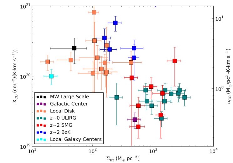Figure 43. Observed XCO determinations vs. galaxy surface density for the Milky Way, local galaxy disks, local galaxy disk nuclei, z ~ 0 ULIRGs, and z ~ 2 SMGs and BzK galaxies. A clear inverse relationship is seen between XCO and ΣH2. Error bars are taken from uncertainties published in original papers; when no uncertainties are available, an error of 0.3 dex is assumed. Data are taken from Oka et al. (1998, MW Galactic Center) Downes & Solomon (1998) (ULIRGs), Weiss et al. (2001), Bolatto et al. (2008), Sandstrom et al. (2013), Donovan Meyer et al. (2012a, 2013) (Local Disks), Magdis et al. (2011), Hodge et al. (2012), Magnelli et al. (2012) Ivison et al. (2013), Fu et al. (2013) (SMGs) and Daddi et al. (2010a), Magdis et al. (2011), Magnelli et al. (2012) (BzK galaxies). The range of Milky Way values is a typical observed range of conversion factors and surface densities for Galactic clouds. We include a factor 1.36 in converting from XCO to αCO.

Concomitant with the observational interest in the conversion factor in the last few years has been a flurry of theoretical activity in the field. Glover et al. (2010) and Glover & Mac Low (2011) utilized magnetohydrodynamic models of GMC evolution combined with chemical reaction networks to show that H₂ can survive in low metallicity environments, while CO can be more easily destroyed. These models were expanded upon by Shetty et al. (2011a, b), who coupled these models with large velocity gradient radiative transfer simulations to explicitly predict the CO emission.

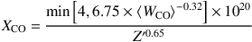
In the regime of large gas surface density, which is more pertinent to the galaxies at hand, Feldmann et al. (2012a) coupled the GMC models of Glover et al. (2010) to a cosmological zoom simula tion of an individual galaxy at z ~ 2. These authors found that at high surface densities, one might expect the X-factor to drop, similar to the empirical findings of Ostriker & Shetty (2011). Narayanan et al. (2011b) and Narayanan et al. (2012a) coupled 3D non-local thermodynamic equilibrium (LTE) radiative transfer calculations and dust radiative transfer simulations with smoothed particle hydrodynamic (SPH) models of disk galaxies and galaxy mergers to derive a functional form for the CO-H₂ conversion factor across a variety of environments. In terms of observables, they derive:

(21)

where ⟨ W_CO ⟩ is the resolved CO surface brightness, and Z′ is the metallicity in units of solar. The idea behind this model is that higher gas velocity dispersions and temperatures in heavily star-forming environments drive up the velocity integrated intensity of the optically thick CO emission line, and thus decrease X_CO = N_H2 / W_CO. Equation 21 predicts a smooth variation in X_CO based on the physical conditions within a galaxy, rather than a bimodality. Obreschkow & Rawlings (2009) applied a Bayesian analysis to literature observational data, and recovered a similar relation between the conversion factor and CO surface brightness, while Ballantyne et al. (2013) evolved analytic models for Eddington-limited starbursts to also find an inverse relationship between X_CO and W_CO. Similarly, Lagos et al. (2012) utilize a semi-analytic model coupled with a photo-dissociation region (PDR) code to investigate the relationship between X_CO, metallicity, UV intensity, and gas surface density. As in other simulation methods, these authors find an inverse correlation between X_CO and Σ_H2.

Though the exact nature of the CO-H₂ conversion factor is unknown in both local and high-z galaxies, significant progress has been made in the last decade. There is still a debate in the literature as to whether the CO-H₂ conversion factor is bimodal or continuous (e.g. Daddi et al., 2010b, Genzel et al., 2010, Narayanan et al., 2012b). This effectively boils down to assuming that the physical conditions in all starburst galaxies are exactly the same (and all normal disk galaxies are exactly the same), versus assuming that there may be dispersion and variation in different galaxies. The ramifications are severe. As we will discuss in the forthcoming subsections, whether one assumes a bimodal X-factor or one that varies with the physical conditions in galaxies has implications for the star formation law (and hence for detailed models for star formation and ISM physics in starburst environments), and whether or not there is disagreement between the observed gas fractions of high-z dusty galaxies and those that derive from theoretical models.

8.3. Star Formation Laws and Efficiencies

Since the original works of Schmidt (1959), and the first major surveys nearly 30 years later by Kennicutt (1989), star formation astrophysicists have sought a physical origin for an empirical form that describes the relation between the star formation rate and gas density. This is usually expressed in terms of the observable surface density terms:

(22)

We will hereafter refer to Equation 22 interchangeably as the “Star Formation Law”, the “Kennicutt-Schmidt (KS) Law”, or the “KS Relation”. We will principally mean the surface density version of the relation, though at times will refer to the volumetric density analog of the equation, and be explicit when doing so. We will refer repeatedly to Figure 44 in this section. In what follows, we first discuss local results, and then expand to results from high-z observations. While the distinction between low and high-z may seem artificial, a few issues related to both gas excitation, and murkiness related to the X-factor arise when considering high-z observations that aren't present in low-z data.

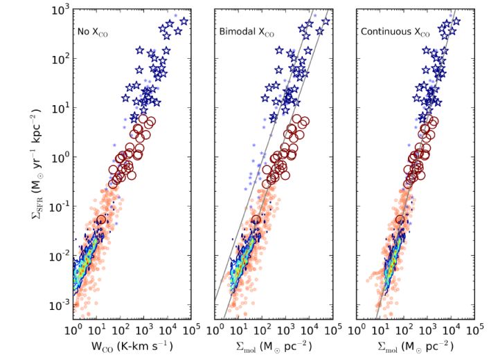Figure 44. Dependence of Kennicutt-Schmidt (KS) star formation relation on assumed CO-H2 conversion factor (XCO). For all plots, the circles represent quiescently star-forming galaxies (galaxies on the SFR-M* main sequence), and stars represent starbursts (galaxies a factor 2-3 above the main sequence). Small orange and blue symbols denote local galaxies, while large magenta and blue symbols denote galaxies at high-z. Contours represent resolved data from Bigiel et al. (2008). Left: KS relation plotting SFR surface density versus CO intensity (i.e. not converting to an H2 gas surface density). Middle: KS relation plotting SFR surface density vs. H2 gas surface density, assuming the traditional bimodal XCO conversion factor. The grey lines denote the best fit sequences to the quiescent galaxies and ULIRGs. This version of the KS relation has given rise to the terminology of multiple 'modes' of star formation (a quiescent mode and a starburst mode). Right: KS relation plotting SFR surface density versus H2 gas surface density, but assuming a smoothly varying XCO conversion factor. The functional form for XCO is that of Equation 21, and can be arrived at either from empirical fits to observations (e.g. Ostriker & Shetty, 2011), or from the results of numerical simulations (Narayanan et al., 2012b). When assuming a smoothly varying XCO (as opposed to a discontinuous one), the star formation relation is unimodal.

The normalization of the relation, є′, reflects the inverse of the gas depletion timescale ¹⁸, and can be thought of as a measure of how easily stars form out of a parcel of gas. Buried in the physics that sets the efficiency are gas depletion, feedback, and turbulence-driven density distribution functions that drive the rate at which stars can form in a given parcel of gas. For example, as we will discuss later in this section, some observational claims point toward ULIRGs and SMGs having an efficiency, є′ a factor ~ 10 greater than disk galaxies. If this is correct, this suggests that a parcel of gas in a ULIRG may form stars at a rate 10 times what is seen in a disk galaxy for the same gas surface density. It is important to note that extragalactic observations typically include many GMCs in a single beam element, and thus care must be taken when the beam filling fraction of clouds may change as a function of galaxy environment.

Similarly, the exponent associated with the KS relation can reveal insight into the underlying small scale physics of star formation, even when considering globally averaged quantities such as single dish galaxy observations. The slope, β is a critical prediction most theories of star formation, and can thus be used as a distinguishing test for different models. For example, Krumholz et al. (2009b) suggest that if the SFR in a galaxy is determined by the fraction of gas in molecular form, the cloud surface density (which occupies a narrow distribution in galaxies like the Milky Way), and turbulence-regulated star formation efficiencies (є), then a linear KS relation is expected (when normalizing by the cloud free fall time, t_ff). On the other hand, in starburst-dominated regimes, where supernova-driven turbulence dominates the velocity dispersion and gas dominates the vertical pressure, Ostriker & Shetty (2011) and Faucher-Giguère, et al. (2013) find an index of ~ 2 should describe the KS relation. These are simply two examples, and there are, of course, a wide range of theories that predict indices ranging from below unity to quadratic (see recent reviews by McKee & Ostriker, 2007, Kennicutt & Evans, 2012). In what follows, we will review recent progress over the last decade in this field, with a particular eye toward high-z galaxies. We refer the reader to the excellent recent review by Kennicutt & Evans (2012) for a more thorough summary of the star formation law in the Milky Way and nearby galaxies.

The seminal study of Kennicutt (1998b) compared the SFR of 36 nearby infrared-selected galaxies against the total gas mass as measured by HI and CO (as a proxy for H₂). Kennicutt derived an index of β = 1.4. Over the following decade, it became clear that the SFR is principally correlated with the H₂ gas in galaxies, and not HI (e.g. Wong & Blitz, 2002). Henceforth, when we refer to the star formation law, we refer to the molecular gas KS relation, and discard any contribution to the gas content from atomic gas.

Utilizing data from the THINGS, HERACLES, and BIMA SONG surveys (Walter et al., 2005, Leroy et al., 2009, Helfer et al., 2003, Bigiel et al. (2008)) investigated the resolved star formation law in nearby galaxies. These authors found that the SFR is principally correlated with H₂ gas (as traced by CO (J = 2-1) in this case), and unassociated with HI in nearby galaxies. This result was extended to the atomic gas-dominated outskirts of nearby galaxies by Schruba et al. (2011). A principle result from these groups is that the SFR is linearly related to the molecular gas surface density on resolved (a few hundred pc) scales, when assuming a constant line ratio from CO (J = 2-1) to (J = 1-0) (with Σ_SFR), as well as a constant X_CO. The results from Bigiel et al. (2008) and Leroy et al. (2008) are denoted by the colored contours in Figure 44. Utilizing a sample of 222 galaxies, Saintonge et al. (2011) found an increasing molecular depletion time scale (where the depletion time scale is the inverse of є′) with galaxy mass, while a roughly constant atomic gas depletion time scale across their mass range of 10 < log M_* / M_⊙ < 11.5.

It should be noted that the claim of a linear KS law when considering normal, quiescent local galaxies has been disputed by a number of groups on varying physical grounds. For example, Liu et al. (2011) argue that when one subtracts the diffuse component from SFR maps, then a super-linear resolved KS relation emerges in NGC 3251 and NGC 5194. On the other hand, Blanc et al. (2009), Shetty et al. (2013a, b) suggest that due to issues related to bisector fitting methods (which have been used in many of the resolved KS relation studies), the true KS slope should be sub-linear. Indeed, there is no consensus on the observed KS slope in galaxies, even when only considering nearby, quiescent systems.

While the numbers of high Σ_SFR galaxies in the local Universe are small as compared to quiescent systems, there appears to be a possible steepening of the KS relation at the transition from normal galaxies to starbursts (ULIRGs). The interpretation of this is muddied by X-factor assumptions, but such a steepening is potentially visible even when considering the KS law in terms of observables themselves. This is apparent in the left panel of Figure 44, where the light orange circles represent local quiescent galaxies, and the light (small) blue stars represent local starbursts. Gao & Solomon (2004b) find a slope of 1.25 - 1.44 between L_IR and L_CO (i.e. pure observables) when considering unresolved CO (J = 1-0) observations of both local quiescent galaxies, and nearby LIRGs and ULIRGs.

If the KS relation steepens from quiescent galaxies to ULIRGs, this may reflect a change in the physical conditions in the ISM in these galaxies, which results in a decreased star formation time scale (or increased inverse depletion time scale, є′). Krumholz et al. (2009b) have posited that perhaps this transition may reflect a regime where GMCs are no longer regulated by internal processes, but rather the external galactic pressure exceeds the internal cloud pressure. It is plausible, in any case, that the compact, warm, and turbulent conditions at the center of a starburst drives different physical conditions in the molecular ISM, and that star formation efficiencies may be enhanced accordingly.

The dramatic increase in the number of CO detections at high-z in recent years (e.g. Carilli & Walter, 2013) have allowed for a significant expansion in the number of high Σ_SFR galaxies, and thus a window into star formation in more extreme environments accordingly, though the interpretation of the results is steeply dependent on the form of the CO-H₂ conversion factor assumed. The first major CO surveys that examined the KS relation at high-z were presented by Greve et al. (2005) and Bouché et al. (2007) which were limited to only the brightest sources (i.e. SMGs). Bouché et al. (2007) found that, when utilizing a local ULIRG-like X_CO conversion factor, the resulting KS relation (including local galaxies as well) was strongly super-linear, with an index of ~ 1.7. A super-linear index in the KS relation suggests that very high Σ_SFR galaxies have shorter gas depletion time scales than lower Σ_SFR galaxies. On the other hand, other studies by Daddi et al. (2010b) and Genzel et al. (2010) suggest that the KS relation may be linear when including high-z galaxies, though these studies additionally include more quiescent galaxies on the SFR-M_* main sequence.

The situation gets potentially murkier when considering high-z systems due to the fact that high lying lines of CO are typically observed, rather than the ground-state transition owing to CO (J=1-0) being redshifted out of typical instrument bandpasses. Krumholz & Thompson (2007) and Narayanan et al. (2008a, c, 2011a) argue that differential excitation in observed KS relation can be strong, and that because high-z galaxies are typically observed in high J transitions, when converting down to CO (J = 1-0), there can be systematic trends in the line ratios with Σ_SFR that will cause the true underlying KS relation to be steeper than what is observed. Certainly, Figure 45 highlights that no single set of line ratios can apply to high-z starbursts, and there is significant dispersion. Whether or not there is a systematic trend with Σ_SFR is at present unclear.

Precisely determining the normalization of the KS law is comparably difficult, and is inextricably tied to a sensitive dependency on the CO-H₂ conversion factor. For example, Daddi et al. (2010b), Genzel et al. (2010) and Bothwell et al. (2010) presented relatively large samples of CO-detected galaxies at high-z. These included both very luminous systems such as SMGs, as well as more moderate star-forming galaxies that lie on the SFR-M_* main sequence. When applying a Galactic CO-H₂ X_CO conversion factor to local disk galaxies, and main sequence galaxies at high-z, and an X_CO a factor 6-8 lower for local ULIRGs and high-z SMGs, a bimodal KS relation emerges. This bimodal relation is comprised of a low star formation efficiency sequence that quiescent star-forming disks at all redshifts live on, and a high star formation efficiency sequence that starbursts live on. This is shown in the middle panel of Figure 44. At face value, the interpretation of this plot is that there are two 'modes' of star formation in galaxies - a quiescent mode and starburst mode. In this physical scenario, two galaxies at a comparable set of gas surface densities may have star formation rate surface densities that vary by an order of magnitude.

A large number of theories have been posited in an attempt to understand the physical nature of the bimodal KS relation, or whether the bimodality is real. Daddi et al. (2010b) and Genzel et al. (2010) advocated a model in which the underlying star formation is driven by large scale dynamical effects, and that if one normalizes by the galaxy dynamical time (i.e. construct a relation: Σ_SFR ∝ Σ_mol / t_dyn), the bimodality disappears. Krumholz et al. (2012) developed a model in which the star formation rate operates on some fraction of the small-scale gas free fall time, and can be parameterized by a relation as in Equation 22. They showed that if one takes plausible values for the typical gas free fall time in galaxy disks, and luminous starbursts, the apparent bimodal relation exhibited in the Daddi et al. (2010b) and Genzel et al. (2010) data reduces to a single, unimodal relation. An alternative class of theories was presented by Ostriker & Shetty (2011), and Narayanan et al. (2012b), who argued that the existence of a bimodal KS relation was an artifact of the usage of a bimodal CO-H₂ conversion factor, and that if a unimodal (either constant, or smoothly varying) X-factor was employed, the KS relation would no longer appear bimodal. Ostriker & Shetty (2011) fit observed data between X_CO and Σ_H2 presented in Tacconi et al. (2008) to derive an empirical form for a smoothly varying X-factor, while Narayanan et al. (2012b) utilized numerical simulations in order to derive a theoretical model form for the conversion factor (Equation 21). After applying their models for a continuously varying CO-H₂ conversion factor, both Ostriker & Shetty (2011) and Narayanan et al. (2012b) found that the bimodal KS relation reduces to a tight, unimodal relation, with index roughly 2. This is represented in the right panel of Figure 44. A yet additional class of models exists that posits that the bimodality is in fact real, and that galaxies undergoing starbursts can go through short periods of extreme star formation efficiency. Teyssier et al. (2010) suggested that, due to extreme amounts of dense gas formed during a merger, a distributed starburst in a galaxy merger may occur with very high efficiency, driving these starbursts through a phase where they reside on the upper normalization of the bimodal KS relation.

The question is not whether or not the KS relation is bimodal, but rather how much dispersion there is in it (e.g. Feldmann et al., 2012b, Freundlich et al., 2013). The apparent bimodality is simply a statement that the inverse depletion time scale can vary by up to an order of magnitude at a given gas surface density. Characterizing how much the star formation efficiency (inverse depletion time scale) can vary, and why, is a fundamental question for both star formation and galaxy evolution astrophysics. Moving forward, detailed studies of both extreme systems at high-z, as well as galactic nuclei in the local Universe that can eliminate some of the uncertainties that have been present in previous surveys may provide some insight.

For example, Fu et al. (2013) utilized both gas to dust ratio constraints, as well as theoretical models in order to constrain X_CO in a detailed study of a SFR ~ 2000 M_⊙ yr^-1 SMG caught in the act of merging at z ~ 2. Given their constraints on the CO-H₂ conversion factor for this particular object, Fu et al. (2013) concluded that the SMG will lie above an extension of the local disk KS relation (though would fall within the mix of high-z galaxies [blue stars] when assuming a smoothly varying X_CO; e.g. the right panel of Figure 44). A similar result was found by Ivison et al. (2013), who employed dynamical constraints on the conversion factor in a comparably luminous source to the Fu et al. (2013) study. Similarly, Leroy et al. (2013) employ a dust to gas ratio-dependent X_CO when studying 1 kpc regions in nearby galaxies, and find that the star formation efficiency toward nearby galaxy centers may increase from the typical field GMC.

In summary, while significant progress has been made in understanding star formation laws as they pertain to high-z dusty galaxies in recent years, the field is still wide open. Even precisely determining the observed slope and dispersion in the relation is an extremely difficult task, though crucial for constraining theories of star formation.

8.4. The Role of Dense Molecular Gas

8.4.1. Physics Learned from the Milky Way and Local Galaxies

Over the last decade, a great deal of effort has been put forth in investigating the role of dense molecular gas in giant molecular clouds and galaxies. This has been motivated by Galactic studies which show a correlation between the dense molecular gas (as traced by high critical density tracers, such as HCN, HCO⁺ and CS), and young stellar objects (e.g. Evans, 1999, and references therein). In contrast, owing to high optical depths in clouds, the relatively low effective density ¹⁹ of CO (n_eff ≈ 10 - 100 cm^-3) means that it traces the bulk of the molecular mass in a cloud (modulo potential metallicity effects; see § 8.2), rather than the sites of active star formation.

In order to investigate the relationship between the star formation rate of galaxies and the dense gas mass, Solomon et al. (1992) and Gao & Solomon (2004a, b) performed the first large extragalactic surveys of HCN in nearby galaxies, targeting normal disks, LIRGs and ULIRGs between an infrared luminosity range of ~ 7 × 10⁹ - 2 × 10¹² L_⊙. These authors found a tight linear relationship between L_IR and L_HCN, suggesting that the star formation rate in galaxies is controlled by dense gas traced by HCN with effective density n > n_eff ≈ 3 × 10⁴ cm ^{- 3}. This result was supported by observations of CO (J = 3-2) from nearby disks, LIRGs and ULIRGs that all found a roughly linear FIR-L_{CO J=3 - 2} relationship (Yao et al., 2003, Narayanan et al., 2005, Iono et al., 2009, Mao et al., 2010).

This interpretation was expanded upon by Wu et al. (2005) and Wu et al. (2010), who extended this study to dense clumps ²⁰ within the Galaxy and found a similarly linear relation between L_IRand HCN luminosity. Complementary work utilizing HCO⁺(J = 3-2), which has a similar effective density as HCN (J = 1-0) (Juneau et al., 2009), as well as high-visual extinction molecular gas as dense gas tracers have found roughly linear dense gas star formation laws for clumps within the Milky Way (Lada et al., 2010, Schenck et al., 2011). Mangum et al. (2008) and Mangum et al. (2013) observe formaldehyde in a sample of nearby disks and starbursts, suggesting a linear relationship between SFR and dense gas mass traced by this molecule is also possible. Wang et al. (2011a) find an slope of 0.94 between L_IR and CS (J = 5-4; n_eff = 2 × 10⁶), and Graciá-Carpio et al. (2006) find a roughly linear slope with HCO⁺ (J = 3-2; n_eff = 6 × 10⁴). These papers forward an interpretation in which there is a volume or surface density threshold for star formation within galaxies, and that dense clumps represent fundamental star formation units. In this scenario, a linear relation between SFR and the mass probed by HCN is natural. Starburst galaxies, then, simply have an increased number of dense star-forming units.

On the other hand, observations of a large number of dense gas tracers show both super-linear and sub-linear star formation laws, casting a shadow on the interpretation that HCN (J=1-0) traces a fundamental star formation unit in galaxies. For example, Bussmann et al. (2008) observed a large subset of the Gao & Solomon (2004a, b) sample in HCN (J = 3-2) (with n_eff = 7 × 10⁵ cm^-3, a factor of ~ 20 larger than the effective density of HCN (J = 1-0)), and found a sub-linear dense gas star formation law with index ~ 0.7 - 0.8. Similarly, Bayet et al. (2009) examined the relationship between SFR and CO emission with transitions ranging from J = 1-0 through J = 12-11, and found decreasing dense gas SFR slopes with increasing J_upper (and, hence, increasing n_eff) such that the SFR-CO (J = 1-0) relation had slope ~ 1.4, the SFR-CO (J = 3-2) relation was roughly linear, and the SFR-CO (J = 12-11) had slope of ~ 0.5. Even the results from HCN (J = 1-0) alone provide a somewhat confusing picture as some groups have found a super-linear relationship between L_IR and HCN (J = 1-0) in local galaxies (García-Burillo et al. 2012). A tentative trend is evident in this series of observations that higher critical density tracers appear to have lower SFR law slopes (Juneau et al., 200). This trend may be evident in Milky Way clumps, though it is tentative. When Wu et al. (2010) examined the robust fits between the SFR and a variety of dense gas tracers, a number of tracers exhibited sub-linear slopes; on the other hand, the least squares fits were typically consistent with slopes of unity.

Theories on the origin of dense gas star formation laws can be broken into three camps: (1) Those that ascribe their origin to the gas density probability distribution function (PDF) in star-forming galaxies; (2) Those that connect a linear dense gas Kennicutt-Schmidt relation to a density or surface density threshold for the onset of star formation; (3) Those that appeal to chemistry models, and the influence of X-ray driven chemistry that owes either to intense starbursts or AGN input.

Models that relate the index of the SFR-line luminosity index for various dense gas tracers to the gas density PDF in galaxies were developed by Krumholz & Thompson (2007) (utilizing analytic models for GMC structure), and Narayanan et al. (2008c) (utilizing hydrodynamic models for galaxies in evolution). In this picture, the principle driver behind the power-law index, β in the SFR-L_mol^β volumetric (gas mass-based) star formation law is the relationship between the gas density distribution and the effective density of the emitting dense gas tracer. A linear HCN (J = 1-0) star formation law simply reflects the relationship between the n_eff of HCN (J = 1-0), and the typical mean density in nearby galaxies. Two testable predictions arise from these models: (1) molecular lines with effective densities higher than HCN (J = 1-0) should have sub-linear star formation law slopes for local galaxies as they trace gas further out in the high-density tail of the density PDF. There may be some indication of sub-linear SFR law slopes for very high effective density tracers (e.g. Bussmann et al., 2008, Graciá-Carpio et al., 2008, Bayet et al., 2009), though larger samples are most certainly necessary. (2) Very high density systems (such as SMGs, or galactic nuclei) should have a super-linear SFR-HCN (J = 1-0) relation (Narayanan et al., 2008a). Indeed, observed increased HCN/CO ratios with galaxy SFR is tentative observational evidence that the gas density PDF is shifting toward higher densities in these systems (Juneau et al., 2009, Rosolowsky et al., 2011). This test will be fully realized with surveys of HCN (J = 1-0) at high-z with the VLA.

An alternative to this picture is the threshold star formation law in which meeting a volume or surface density threshold is a prerequisite to beginning the star formation process. Lada et al. (2010) find roughly linear relationships between SFR and gas above an extinction threshold of A_K ≈ 0.8 mag in Galactic clumps, a result consistent with the work of Heiderman et al. (2010). These authors argue that this is comparable to a threshold surface density of ~ 100 M_⊙ pc ^{- 2}, which is roughly equivalent to a volume density threshold of ~ 10^4-5 cm^-3, depending on the cloud geometry. An attractive aspect of this picture is that the density threshold is roughly matched with the density probed by HCN (J = 1-0). This scenario suggests that HCN traces the dense gas that more actively forms stars better than CO, and thus predicts an SFR relation with lower dispersion. Wu et al. (2010) interpret the roughly linear relations between SFR and different dense gas tracers in their study of Galactic clumps as further evidence for this model.

A third class of models appeals to chemistry driven by X-rays in the vicinity of high star formation rate surface density environments, or an AGN (e.g. Lintott & Viti, 2006, Meijerink et al., 2013). At least some evidence for this has been seen by Krips et al. (2008) and Graciá-Carpio et al. (2008) in nearby active systems.

8.4.2. Dense Gas at High-Redshift

The study of dense gas at high-z is at its infancy, though it holds great promise for constraining models of star formation owing to the extreme gas physical conditions in SMGs. Gao et al. (2007) studied HCN (J = 1-0) in a sample of high-z SMGs and quasars, finding a relationship between the FIR luminosity in these systems and HCN luminosity, though offset from the local one (such that the high-z points lie above the local linear relation). It is unclear whether this owes to higher gas density PDFs (e.g Krumholz & Thompson, 2007, Narayanan et al., 2008c), or contribution to the FIR luminosity by AGN. Further evidence for a nonlinear FIR-HCN trend in dense, high-z systems was provided by Greve et al. (2006) and Riechers et al. (2007).

Other well-studied sources include the Cloverleaf quasar (e.g. Solomon et al., 2003 and APM 0829+5255 (Wagg et al., 2005, Riechers et al., 2010b). These sources are both lensed, however, which adds the additional potential complicating factor of differential magnification. On average, a consensus finding from dense gas observations in high-z SMGs is that these systems tend to have a larger fraction of their ISM in a dense phase than local field galaxies. Further evidence for this is seen in the high-excitation CO SLEDs that are typical of these sources (Carilli & Walter, 2013, Riechers et al., 2013b). Future surveys of HCN (J = 1-0) from high-z SMGs, and comparisons to low-z relations will provide valuable insight into the physical conditions that govern star formation (e.g. Krumholz & McKee, 2005, Andrews & Thompson, 2011, Hopkins et al., 2013e). Obtaining large samples of dense gas emission lines from galaxies at high-z is an important priority for the coming decade.

Alongside dense gas tracers HCN and HCO⁺, observations of water have been gaining traction in the past few years. The rotational transitions of H₂O have very high critical densities (~ 10⁸ cm^-3), and therefore only happen in the extremely dense parts of star-forming clouds. The bulk of studies thus far have focused on low-z systems (e.g. Yang et al., 2013), though at least a few have attempted to push to higher redshifts. The early studies typically detected water masers (e.g. Barvainis & Antonucci, 2005, Impellizzeri et al., 2008), though in recent years, non-masing sources at high-z have been procured as well (Omont et al., 2011, 2013). Riechers et al. (2013b) impressively detected seven H₂O lines in the z = 6.34 galaxy HFLS3. A key result from these studies is that a clear correlation between H₂O luminosity and infrared luminosity exists a range L_IR ~ 10¹² - 10¹⁴ L_⊙. Omont et al. (2013) find a relation L_H2O ∝ L_IR^1.17.

8.5. CO Excitation and Spectral Line Energy Distributions

The CO spectral line energy distribution (CO SLED; alternatively known as the CO rotational ladder) from a galaxy provides a unique window into the bulk physical properties of the molecular gas in a given system. The SLED describes the relative strengths of CO emission lines, and reveals the level populations of CO molecules. Typically, the CO SLED of a galaxy is represented as the CO line intensity versus the rotational level of the line. The excitation of CO is dependent on the gas density and temperature (along with secondary effects, including the line optical depth). Generally, the relative excitation of two transitions of CO can be expressed as a ratio of of brightness temperatures, line luminosities or line intensities.

Typically, the warmer and denser a system, the more heavily populated the upper levels will be. For a system that is in local thermodynamic equilibrium (LTE) such that the levels can be described by Maxwell-Boltzmann statistics, the line intensity is given by the Planck function, and for warm enough temperatures (such that E_upper << kT), the SLED will rise as the square of the line frequency ²¹. Typically, these systems are referred to as 'thermalized', or 'thermal', and level populations that fall below what is expected for LTE are 'sub-thermal'. While observing high-J CO lines in local galaxies has been difficult in the pre-Herschel and ALMA years, observations of high-z SMGs have routinely been deriving well-sampled CO line ladders owing to the redshifting of submillimeter-wave lines into atmospherically favorable observing windows.

Constraining the CO SLED for galaxies has two main purposes. First, armed with a radiative transfer code (such as an escape probability code, or large velocity gradient (LVG) code; e.g. Krumholz, 2014), with multiple CO emission lines one can constrain the combination of temperatures and densities necessary to drive the observed CO excitation. This requires some assumption about the CO abundance and typical velocity gradient in emitting GMCs. Second, at high-z, most detections of CO are of high-lying transitions. In order to derive the total gas mass as traced by CO (J = 1-0) (see § 8.2), one needs some knowledge regarding the CO excitation.

Because high-z SMGs are the most extreme star-forming galaxies in the Universe, it has long been assumed that LTE is a safe assumption for the level populations. Indeed, local starburst galaxies such as M 82 and NGC 253 exhibit CO SLEDs that are nearly thermal out through J ~ 5 (Weiss et al., 2005, Hailey-Dunsheath et al., 2008). However, early detections of CO (J = 1-0) with the Green Bank Telescope (GBT) and VLA revealed that SMGs appear to exhibit a diverse range of CO SLEDs, and that at least some SMGs may indeed contain large volumes of sub-thermally excited gas (e.g. Greve et al., 2003, Hainline et al., 2006, Carilli et al., 2010, Harris et al., 2010, Ivison et al., 2011). Still, other SMGs show rather extreme conditions, and appear to have thermalized level populations through the J = 6-5 transition (e.g. HFLS3, Riechers et al., 2013b). We quantify the diversity of CO SLEDs from high-z SMGS in Figure 45, where we show the CO SLEDs for all bona fide SMGs that have a CO (J = 1-0) detection. For reference, we also show the rotational ladder for the Galaxy, M 82, and what is expected for thermalized level populations so long as E_upper << kT.

Figure 45. CO Spectral Line Energy Distribution (SLED) for high-redshift SMGs (black lines) that have a CO (J = 1-0) detection. In cases of multiplicity, the SLED is for the composite system, unless the individual components also satisfy the SMG criteria (S850 > 5 mJy). Galaxies are only ones that have CO 1-0. For reference, the SLED for the Milky Way is shown (red line, Fixsen et al., 1999), as well as M 82 (Weiss et al., 2005, purple line), and what is expected for LTE (blue line). As is apparent, there is a large diversity in SMG CO SLEDs, ranging from nearly thermalized through J = 6, through sub-thermal even at the J = 3-2 line. The CO SLEDs are taken from Andreani et al. (2000), Aravena et al. (2010, 2012), Baker et al. (2004), Bothwell et al. (2013a), Carilli et al. (2010), Danielson et al. (2011), Downes & Solomon (2003), Fu et al. (2013), Greve et al. (2003, 2005), Hainline et al. (2006), Harris et al. (2010), Ivison et al. (2011, 2013), Neri et al. (2003), Papadopoulos & Ivison (2002), Rawle et al. (2013), Riechers et al. (2011d, 2013b), Scott et al. (2011), Sharon et al. (2013), Weiss et al. (2009a), and the Milky Way SLED was provided by Chris Carilli and Fabian Walter (private communication). By and large, most SMGs are thermalized through the J = 2-1 transition, and many through the J = 3-2 transition. However, assuming constant brightness temperatures at Jupper ≥ 3 for high-z SMGs is a poor assumption. Note, however, that the Cloverleaf and APM 0829 are lensed, and differential amplification is a major concern if different gas reservoirs have different sizes, which in turn affects their excitation. Similarly, HFLS3 has to be intrinsically hotter to be detected at z≈6, an important selection effect to consider.

Two salient points are clear from Figure 45. First, based on the physical characterization of their ISM properties alone, SMGs appear to be a heterogeneous galaxy population. While some galaxies have CO excitation patterns consistent with very warm and dense gas, others have much weaker excitation. This may be consistent with theories that suggest that SMGs may be made up of both merger-induced starbursts caught at final coalescence (that may have more extreme ISM conditions), as well as individual disk galaxies at high-z that may have a lower-excitation ISM (e.g. Hayward et al., 2011, 2012, 2013b). Indeed, some observations of SMGs support this picture (Hodge et al., 2013b, Karim et al., 2013).

Second, it is clear that there are no 'average' line ratios for SMGs. The ladders are diverse, with line ratios at a given transition differing, at times, by an order of magnitude. This level of uncertainty can be comparable to what is present in the CO-H₂ conversion factor, and should be reflected in any H₂ mass measurements derived from down-converting high-excitation CO lines to the 1-0 transition. In an effort to reduce this uncertainty, Narayanan & Krumholz (2014) developed a model in which the the CO SLED is controlled by difficult-to-observe parameters such as the gas density, temperature, and line optical depths. However, these physical quantities scale well with the global galaxy SFR surface density. As a result, Narayanan & Krumholz (2014) were able to derive a power-law parameterization for the CO excitation as a function of Σ_SFR. Going forward, other theoretical or empirical calibrations for the SLED in terms of an observable proxy will be useful for interpreting high-z data.

Finally, a number of recent works have pointed out that modeling high-z dusty systems as single phase (single T and ρ) provides a poor fit to the observed SLED. For example, Harris et al. (2010), Riechers et al. (2011c) and Hodge et al. (2013a) find that some SMGs are best modeled with both a compact, high-excitation phase, as well as a more extended diffuse ISM. This is in contrast with high-z quasar host galaxies, which can typically be modeled as dominated by a single high-excitation gas component (e.g. Riechers et al., 2011a, Weiss et al., 2007).

8.6. Molecular Gas Fractions

One of the most remarkable aspects of high-z dusty galaxies is their incredibly large gas fractions as compared to present-epoch galaxies. The gas fraction, defined here as:

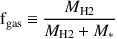(25)

considers the fraction of baryons in a galaxy that is in molecular form, neglecting any contribution from HI. It is likely, however, that in the high-pressure environments typical of starburst galaxies, that the bulk of the hydrogen in the ISM is in molecular form (Blitz & Rosolowsky, 2006, Krumholz et al., 2009a). Measurements of high-z star forming galaxies (ranging from relatively quiescent BzK galaxies, forming at ~ 10 - 100 M_⊙ yr^-1, to dusty starbursts), suggest gas fractions ranging from f_gas ~ 0.2 - 0.8 (e.g. Daddi et al., 2010a, Tacconi et al., 2010, Geach et al., 2011, Magdis et al., 2012b, Combes et al., 2013, Tacconi et al., 2013). This is to be compared to local galaxies, which show typical gas fractions f_gas < 10% (e.g. Saintonge et al., 2011). These results have come from both from CO inferred H₂ gas masses, as well as dust measurements and associated dust-to-gas ratio assumptions (Magdis et al., 2012a).

While no study has performed a proper mass-selected study, indications from these observations are that the average gas fraction of galaxies rises toward high-redshift. This general trend is in good agreement with cosmological galaxy formation simulations (e.g. Bouché et al., 2010, Dutton et al., 2010, Lagos et al., 2011, Davé et al., 2012). In galaxy formation theory, the baryonic gas fraction is set by a balance between gas accretion from the intergalactic medium (IGM), and the removal of gas by star formation and galactic outflows (with small perturbations from stellar mass loss and recycled gas outflows Oppenheimer et al., 2010). At higher redshifts, the baryonic inflow rate, which scales strongly with redshift (e.g. Dekel et al., 2009a, Fakhouri et al., 2010), ensures that large gas reservoirs are built up in galaxies. Geach et al. (2011) suggest that an evolution in M_gas / M_* ²² with redshift as M_gas / M_* ∝ (1 + z)^{2 ± 0.5} provides a reasonable fit to observed data.

On average, galaxy gas fractions decrease with increasing stellar mass. This point has been predicted in theoretical models (e.g. Davé et al., 2010, 2011, Lagos et al., 2011, Popping et al., 2012, 2013), as well as observationally confirmed (Combes et al., 2013, Saintonge et al., 2013, Tacconi et al., 2013, Santini et al., 2013). This trend is additionally seen in low-redshift galaxies, though Saintonge et al. (2011) suggest that the gas fractions of low-z galaxies are more closely correlated with stellar density than stellar mass. We see this quantitatively for high-z SMGs in Figure 46, where we plot the gas fraction for all SMGs with CO (J = 1-0) detections (to minimize the relatively large uncertainty in CO excitation; c.f. § 8.5). We use a conversion from CO to H₂ assuming α_CO = 0.8 for high-z SMGs, and α_CO = 4 for BzK galaxies, despite the likely problems associated with assumption outlined in § 8.2.

Figure 46. Molecular gas fraction as a function of stellar mass for SMGs (red points). These are compared to theoretical models by Benson (2012), Lagos et al. (2012), Fu et al. (2012b), Popping et al. (2013) and Davé et al. (2012). The red shaded region shows the approximate region spanned by the observations. The models span a range of methods, from bona fide cosmological hydrodynamic simulations to four different Semi-Analytic prescriptions. By and large, inferred gas fractions of observed high-z galaxies are all a factor of a few larger than any theoretical model predicts. The observed gas fractions are computed assuming a CO-H2 conversion factor of αCO = 0.8 for SMGs, and αCO = 4 for BzK galaxies, which, for better or worse, is the canonical assumption in the literature. Given the large spread in potential CO excitation (c.f. § 8.5), we only consider galaxies with CO (J = 1-0) detections to remove the uncertainty in down-converting high-excitation lines to the ground transition. The CO (J = 1-0) measurements were reported by Aravena et al. (2010, 2012), Baker et al. (2004), Bothwell et al. (2010, 2013a), Carilli et al. (2010), Daddi et al. (2010a), Fu et al. (2013), Greve et al. (2003), Hainline et al. (2006), Ivison et al. (2011, 2013), Scott et al. (2011), Sharon et al. (2013), Swinbank et al. (2011), Riechers et al. (2011c, 2013b).

This said, there is some tension between galaxy formation models and observed gas fraction in galaxies. Generally, most galaxy formation models predict galaxy gas fractions at a given mass a factor of a few lower than what is observed (e.g. Bouché et al., 2010, Dutton et al., 2010, Fu et al., 2012b, Haas et al., 2013, Davé et al., 2012). What is particularly disconcerting about this disagreement is that these models utilize a wide - range of modeling techniques: the problem is pervasive in galaxy formation theory. This is clear from Figure 46, where we show the model predictions of several groups (Benson, 2012, Lagos et al., 2012, Fu et al., 2012b, Davé et al., 2012, Popping et al., 2013) in comparison to observational determinations. This implies either a fundamental problem in our theoretical understanding of how galaxies grow over cosmic time, or an issue in our calculation of gas masses in high-z galaxies.

One possible solution to this mismatch has been offered by Narayanan et al. (2012a), who suggested that the canonical “ULIRG” conversion factor (α_CO = 0.8) was too large for the most extreme systems at high-redshift, and that the gas temperatures and velocity dispersions were high enough to warrant even lower conversion factors. Recalling § 8.2, these authors suggested that if one uses either an empirically derived form for α_CO from Ostriker & Shetty (2011), or the theoretically derived continuous form for α_CO from Narayanan et al. (2012b) (Equation 21), typical conversion factors for SMGs will range from ~ 0.3 - 0.5. In this case, there can be reconciliation between the gas fractions of many observed SMGs, and the gamut of theories that predict lower gas fractions. Interestingly, there is at least one observed case of an massive (M_* ≈ 2 × 10¹¹ M_⊙ ) SMG that exhibits a high gas fraction f_gas ~ 50%, even when considering the aforementioned models for α_CO (Fu et al., 2013).

An alternative theoretical solution has been suggested by Gabor & Bournaud (2013), who utilized a combination of analytic arguments and high-resolution numerical simulations to show that star formation in galaxies undergoing heavy accretion from the IGM may be delayed owing to energy input into the disk from the accreted gas. The increase in turbulence driven by the accreted gas reduces the star formation efficiency, and allows gas fractions to rise accordingly (though see Hopkins et al., 2013b for counter arguments).

Finally, Tacconi et al. (2013) suggest that the tension between galaxy gas fractions measured in observations and simulated galaxies may owe to incompleteness in the observations. In particular, when correcting for incomplete sampling of galaxies in the SFR - M_* main sequence (owing to SFR cuts), the observed gas fractions can come down in better agreement with cosmological simulations.

Going forward, a key advance will be to construct a large enough sample of galaxies at high-redshift within narrow stellar mass bins in order to derive reliable measurements of the evolution of galaxy gas fractions (at a given stellar mass) with redshift.

8.7. Molecular Gas Morphology and Dynamics

Over the past decade, the advent of (sub)mm-wave interferometers, and increased capabilities of radio-wave interferometers have allowed for meaningful samples of CO, FIR, and radio morphologies of high-z dusty galaxies. Here we discuss morphology and dynamics from CO, in contrast to the earlier discussions provided in § 5. The CO spatial extent can constrain the H₂ gas surface density, which aids in placing a galaxy on the Kennicutt-Schmidt star formation relation (c.f. § 8.3). Molecular and atomic line dynamics can provide information regarding the physical origin of a galaxy (i.e. if it is a dynamically hot, as one might expect from a merger, or dynamically cold), and in the cases of multiple CO lines, can even provide a map of the thermal and density structure in high-z galaxies.

High-resolution observations with the PdBI, VLA and ALMA interferometers have afforded detailed studies of the molecular gas morphology as traced by various CO transitions in high-z SMGs. Molecular line morphologies give both a measure of the emitting-region size for gas surface density measurements, as well as an idea of the dynamics of the gas. As discussed in § 8.5, the excitation of CO in high-z starburst galaxies is relatively diverse, meaning that different transitions can, at times, trace different spatial extents. In Figure 47, we plot the ratio of the sizes of the FWHM CO line widths of the CO (J = 1-0) and CO (J = 3-2) emission lines for all high-z dusty galaxies where both measurements are available. While the line width is not a measure of the emission size directly ²³, it does reflect a combination of the mass enclosed in the emitting region and the spatial extent of the gas. Though the sample sizes are small, some features are clear. The majority of sources have similar line widths in the CO (J = 1-0) transition, and the denser gas tracer, CO (J = 3-2), though there is a clear high ratio tail where the CO (J=1-0) line width is roughly 10 - 50% larger than the CO (J = 3-2) emitting region. This effect is expected to be more dramatic when considering even higher-lying transitions (which are often probed in high-redshift galaxies due to a combination of telescope instrumentation and the desire for the highest spatial resolution studies possible). Care must be taken when interpreting results that depend on CO dynamics that derive from high-lying lines.

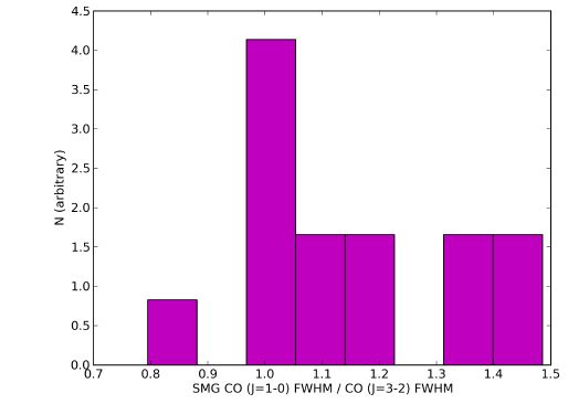Figure 47. CO J = 1-0 / CO J = 3-2 line width ratios. The power toward high ratios suggests stratification in the gas density, temperature or volume filling factor, and hence, CO emitting region for high-J lines. The data are compiled from the Carilli & Walter (2013) compendium.

The molecular gas that has been mapped in normal disk-like galaxies at high-z tends to be extended, compared to local starbursts. This is notable because the global SFRs of high-z disks can oftentimes be comparable to those of compact nuclear starbursts in the local Universe (Daddi et al., 2005). Aravena et al. (2010) and Daddi et al. (2010a) find that BzK galaxies are extended on scales of ~ 6 - 10 kpc (FWHM) in the CO (J = 1-0) and (J = 2-1) transitions. Tacconi et al. (2013) find CO (J = 3-2) sizes (R_1/2) for a large sample of z ~ 1-2 disks ranging from 4-10 kpc, and a reasonable match between the CO size and the optical/UV size.

Turning to starbursts, the number of bona fide CO (J = 1-0) detections of high-z dusty starbursts are few, owing to the lack of sensitive radio interferometers preceding the VLA. Utilizing the VLA, Ivison et al. (2011) found CO (J = 1-0) FWHM sizes of ~ 16 kpc from a sample of SMGs, distinctly more extended than the ~ 1 - 3 kpc half-light radii derived from higher-J lines by Tacconi et al. (2008). Similarly, Riechers et al. (2011c) find source radii of ~ 3 - 15 kpc in a sample of 3 SMGs detected in CO (J = 1-0), and note again that these sizes are notably more extended than the CO (J = 4-3) and (J = 6-5) sizes measured by Engel et al. (2010) for the same galaxies. Interestingly, Riechers et al. (2011a) inferred, based on CO line ratios, that the J = 1-0 emitting region from a sample of quasar host galaxies at similar redshifts to the aforementioned SMG studies (z ~ 2) is relatively compact. One could use this data to argue that QSOs and SMGs derive from distinctly different galaxy populations (though would have to reconcile the similar clustering measurements; Hickox et al., 2012), or that quasars derive from SMGs after undergoing a size transformation (as might be expected from a galaxy merger). We emphasize that the radii for many SMGs that have extended CO (J = 1-0) sizes are ≲ 4 kpc when probing higher lying transitions (Downes & Solomon, 2003, Genzel et al., 2003, Neri et al., 2003, Tacconi et al., 2006, 2008). Note also that these differential sizes for high-excitation gas reservoirs can also exist in quasars, a problem which could be exacerbated in lensed sources due to differential amplification. The differences in source radii likely derive in part from a density or excitation stratification in the gas, but also in part from a genuine diversity in the source population.

One of the principle results of high-resolution CO mapping of starbursts at high-z has been for studies of the dynamics of the gas. Maps of exquisite resolution of z ~ 1-2 disks have provided the first clear evidence for ordered rotation and galaxy disks at high-z (Genzel et al., 2003, Daddi et al., 2010a, Tacconi et al., 2010, 2013). A large step forward was made by Tacconi et al. (2010), who presented a rotation curve out to ~ 8 kpc from the galaxy's center of a z ~ 1 disk galaxy, then from Swinbank et al. (2011) who presented the disk-like kinematics in the Cosmic Eyelash at z = 2.3 (see § 6.2).

For higher-luminosity (starburst) systems at high-z, the main thrust for obtaining CO-based dynamics has been with the motivation of understanding whether or not these systems owe their extreme luminosities and star formation rates to galaxy mergers, or whether they may result from secular processes within a galaxy disk. The results are varied. Some observations have found clear evidence for rotating molecular disks in even extremely bright SMGs and quasars (e.g Tacconi et al., 2008, Bothwell et al., 2010, Carilli et al., 2010, Hodge et al., 2012;, Deane et al., 2013), while other studies have found more seemingly disrupted systems when examining the velocity contours (Tacconi et al., 2008, Engel et al., 2010, Bothwell et al., 2013a, Riechers et al., 2011b, 2013b). Still other groups have shown potentially extremely convincing evidence for ongoing mergers at high-z by showing multiple counterparts that are potentially two galaxies caught in the act of merging, prior to final coalescence (e.g. Engel et al., 2010, Yan et al., 2010, Riechers et al., 2011a, Ivison et al., 2013, Fu et al., 2013). This said, there are reasonable counter-arguments to each of these examples. For example, numerical simulations by Springel & Hernquist (2005) and Hopkins et al. (2009) have shown that very gas-rich mergers at high-redshift can quickly re-form a gaseous disk soon after the merger, due to the dissipational nature of gas.

Narayanan et al. (2009) showed that for the specific example of galaxy mergers massive enough to form luminous systems comparable to observed SMGs, the synthetic CO velocity contours would show signs of ordered rotation some fraction of the time. Thus, observed rotational signatures in high-z systems do not rule out galaxy mergers. Similarly, Davé et al. (2010) showed that SMGs that are fueled primarily from accretion from the IGM (rather than via major mergers) could still show somewhat disrupted disks, due to the sporadic nature of gas accretion.

Finally, even the seemingly clear-cut case of seeing a Also, the impact of the galaxy merger in driving the observed luminosity is potentially minimal (Narayanan et al., 2009, 2010a, Lanz et al., 2013). As an anecdotal example, a distant observer may consider the Milky Way and Andromeda as a pair of galaxies undergoing a merger (depending on the line of sight), yet neither is a “merger-induced starburst galaxy”. The ramifications of these sorts of studies are indeed important. Theoretical models aiming to quantify what fraction of galaxies at a given luminosity are galaxy mergers versus disks produce a wide range of answers (e.g. Baugh et al., 2005, Davé et al., 2010, Dekel et al., 2009a, Narayanan et al., 2010a, Hopkins et al., 2010, González et al., 2011, Hayward et al., 2013b), and any observational constraints in this area are quite valuable (we discuss this issue in more detail in § 10).

What is clear, at present, is that SMGs appear to be a diverse population with respect to their gas kinematics. Clear examples for ordered rotation, non-Keplerian dynamics, and multiple counterparts potentially prior to merging exist. From the dynamical information alone, the submillimeter selection appears to cull a diverse set of systems from high-z galaxies.

Going forward, perhaps one of the most exciting avenues in CO morphology studies of high-z systems will be detailed studies of the ISM in gravitationally lensed systems, comparable to the exquisitely imaged Cosmic Eyelash (see § 6.2) galaxy by Swinbank et al. (2010) and Swinbank et al. (2011). High-redshift galaxies allow for a unique opportunity to study star formation and ISM structure in a much higher-pressure environment than our own galaxy, and may give clues as to how star formation proceeds in galaxies ranging from local ULIRGs through the most extreme starbursts at high-redshift. Swinbank et al. (2010, 2011) found that in the high-pressure environment of the Eyelash, GMCs lie off of local cloud scaling relations (i.e. “Larson's Laws”), and that at a given cloud radius, the GMCs in the Eyelash has higher velocity dispersion. Interestingly, this is also true for massive, dense clumps in our galaxy (Shirley et al., 2003, and references therein).

These sorts of constraints on the basic physical properties of the ISM in these extreme environments can have significant impact in both the astrophysics of star formation and galaxy evolution. For example, models that invoke a variety of physical mechanisms, from accretion and star formation (Goldbaum et al., 2011) to stellar feedback (Hopkins et al., 2012c, Krumholz et al., 2014) in setting the basic properties of molecular clouds will be impacted by our understanding of the structure of the ISM in these test cases. Similarly, nearly every model for the origin and potential variations in the IMF depend on the physical properties of the molecular ISM on small scales (e.g. Krumholz, 2011b, Hopkins, 2013, Padoan & Nordlund, 2002, Narayanan & Davé, 2012, 2013). Because the exact form of the IMF impacts stellar mass estimates, star formation histories, the generation of stellar winds, and interstellar, circum and intergalactic metal enrichment (e.g. Arrigoni et al., 2010, Weidner et al., 2013), these sorts of studies can be impactful on a large range of scales.

8.8. Synthesis

This is a particularly exciting time for high-redshift star formation and molecular gas studies. With the advent of ALMA, as well as substantial upgrades to other ground based facilities (such as the JVLA and PdBI), we are able to detect molecular lines at high-z in a fraction of the time that was previously required. Similarly, numerical simulations are reaching a point where they can resolve giant molecular clouds on galaxy-wide scales.

Going forward, it will be critical to place strict constraints on the major uncertainties in molecular line observations. These include a comprehensive picture (either a theoretical model, or observed empirical relations) for the CO-H₂ conversion factor, as well as the conversion from high-J CO states to low J states.

At the same time, we are lacking a comprehensive understanding of the relationship between the physical state of the ISM, and how star formation subsequently proceeds. How do the density, temperature, and velocity dispersion PDFs affect molecular cloud star formation rates and the initial mass function of stars formed? What is the physical structure of the ISM in high-z galaxies, and how does this impact ongoing star formation? Observations of lensed high-redshift galaxies at high resolution will help elucidate some of these issues. Similarly, observations of both molecular clouds in the Milky Way, and more extreme regions in the local Universe hold great promise for resolving outstanding issues in high-redshift star formation.

¹⁸ є′ is often referred to as the 'star formation efficiency', and should be distinguished from alternative definitions for the star formation efficiency that appear in the literature as well:

(23)

where M_* is the stellar mass formed in a cloud, and M_GMC is the mass of the parent cloud.

(24)

where M_* is the SFR within a galaxy, and M_grav is the gas accretion rate onto the halo from the IGM. In the extragalactic literature, the star formation efficiency (SFE) most often means the inverse depletion timescale (є′), though the reader should take care as the definition from paper to paper will not always be consistent. In what follows, we will be explicit in our terminology for star formation efficiency. Back.

¹⁹ As a reminder, as discussed in Evans (1999), while a density of n > n_crit is usually taken to be necessary for line emission, a variety of effects associated with radiative transfer can affect the observed line strength at a given density. Following Evans, we choose to state, rather than the critical density, the effective density (n_eff, which is defined as the density at which a transition will have a radiation temperature of 1 K, assuming log (N / Δv) = 13.5, and T = 10 K. A table converting n_crit (which is typically 1-2 orders of magnitude higher than n_eff) and n_eff for a variety of molecular transitions is given in Evans (1999) and Reiter et al. (2011). Back.

²⁰ In keeping with the standard definitions in the star formation literature, we will define “clumps” as ~ 1 pc entities within GMCs that may form stellar clusters, and “cores” as ~ 0.1 pc structures that serve as the precursors of individual or binary stars (e.g. Kennicutt & Evans, 2012). Back.

²¹ As shown by Narayanan & Krumholz (2014), the Rayleigh-Jeans condition is not easily met for high J (J≳ 6 CO emission lines), even for extreme starbursts. Back.

²² Note, this is different than our nominal definition of f_gas (Eq. 25). Back.

²³ We choose to use the line width as a proxy for the emitting region size for two reasons. First, it removes any ambiguity as to how a size is defined from one study to another. Second, the sample size of galaxies that have direct morphology measures of multiple CO transitions is incredibly small. Back.