


7.2 Linear Fits. The Straight Line
In the case of functions linear in their parameters aj, i.e., there are no terms which are products or ratios of different aj, (71) can be solved analytically. Let us illustrate this for the case of a straight line
where a and b are the parameters to be determined. Forming
S, we find
Taking the partial derivatives with respect to a and b, we
then have the equations
To simplify the notation, let us define the terms
Using these definitions, (76) becomes
This then leads to the solution,
Our work is not complete, however, as the errors on a and
b must also be
determined. Forming the inverse error matrix, we then have
Inverting (80), we find
so that
To complete the process, now, it is necessary to also have an idea of
the quality of the fit. Do the data, in fact, correspond to the
function f(x) we have assumed? This can be tested by means of the
chi-square. This is just the value of S at the minimum. Recalling
Section 2.4, we saw that if the data
correspond to the function and
the deviations are Gaussian, S should be expected to follow a
chi-square distribution with mean value equal to the degrees of
freedom,
which should be close to 1 for a good fit.
A more rigorous test is to look at the probability of obtaining a
An equally important point to consider is when S is very small. This
implies that the points are not fluctuating enough. Barring falsified
data, the most likely cause is an overestimation of the errors on the
data points, if the reader will recall, the error bars represent a
1
Example 6. Find the best straight line through the following measured
points
Applying (75) to (82), we find
To test the goodness-of-fit, we must look at the chi-square
for 4 degrees of freedom. Forming the reduced chi-square,
Example 7. For certain nonlinear functions, a linearization may be
affected so that the method of linear least squares becomes
applicable. One case is the example of the exponential, (69), which
we gave at the beginning of this section. Consider a decaying
radioactive source whose activity is measured at intervals of 15
seconds. The total counts during each period are given below.
What is the lifetime for this source?
The obvious procedure is to fit (69) to these data in order to
determine
Setting y = ln N, a = -1/
Using (75) to (82) now, we find
The lifetime is thus
The chi-square for this fit is
While the above fit is acceptable, the relatively large chi-square
should, nevertheless, prompt some questions. For example, in the
treatment above, background counts were ignored. An improvement in our
fit might therefore be obtained if we took this into account. If we
assume a constant background, then the equation to fit would be
Fig. 7. Fit to data of Example 7. Note that
the error bars of
about 1/3 of the points do not touch the fitted line. This is
consistent with the Gaussian nature of the measurements. Since the
region defined by the errors bars (± 1
Another hypothesis could be that the source has more than one decay
component in which case the function to fit would be a sum of
exponentials. These forms unfortunately cannot be linearized as above
and recourse must be made to nonlinear methods. In the special case
described above, a non-iterative procedure
[Refs: 2,
3,
4,
5,
6] exists which
may also be helpful.
 where
where
 . In the above problem,
there are n independent data points
from which m parameters are extracted. The degrees of freedom is thus
= n - m. In the case
of a linear fit, m = 2, so that = n - 2. We
thus expect S to be close to =
n - 2 if the fit is good. A quick and
easy test is to form the reduced chi-square
. In the above problem,
there are n independent data points
from which m parameters are extracted. The degrees of freedom is thus
= n - m. In the case
of a linear fit, m = 2, so that = n - 2. We
thus expect S to be close to =
n - 2 if the fit is good. A quick and
easy test is to form the reduced chi-square

 2
value greater than S, i.e., P(2
2
value greater than S, i.e., P(2  S). This
requires integrating the
chi-square distribution or using cumulative distribution tables. In
general, if P(2
S) is greater than 5%, the
fit can be accepted.
Beyond this point, some questions must be asked.
S). This
requires integrating the
chi-square distribution or using cumulative distribution tables. In
general, if P(2
S) is greater than 5%, the
fit can be accepted.
Beyond this point, some questions must be asked.
 deviation, so that about 1/3 of the data points should, in fact, be
expected to fall outside the fit!
deviation, so that about 1/3 of the data points should, in fact, be
expected to fall outside the fit!
x 0 1 2 3 4 5
y 0.92 4.15 9.78 14.46 17.26 21.90
0.5 1.0
0.75 1.25 1.0 1.5
(a) = 0.044
(b) = 0.203 and
2 = 2.078
2 /
 0.5,
we can see already that his is a good fit. If we calculate the
probability P(2 >
2.07) for 4 degrees of freedom, we find P
97.5%
which is well within acceptable limits.
0.5,
we can see already that his is a good fit. If we calculate the
probability P(2 >
2.07) for 4 degrees of freedom, we find P
97.5%
which is well within acceptable limits.
t [s] 1 15 30 45 60 75 90
105 120 135
N [cts] 106 80 98 75 74 73
49 38 37 22
 . Equation (69), of
course, is nonlinear, however it can be
linearized by taking the logarithm of both sides. This then yields
. Equation (69), of
course, is nonlinear, however it can be
linearized by taking the logarithm of both sides. This then yields
 and b = ln N0, we see that this is just a
straight line, so that our linear least-squares procedure can be used.
One point which we must be careful about, however, is the errors. The
statistical errors on N, of course, are Poissonian, so that
(N) =
and b = ln N0, we see that this is just a
straight line, so that our linear least-squares procedure can be used.
One point which we must be careful about, however, is the errors. The
statistical errors on N, of course, are Poissonian, so that
(N) =
 N. In the fit, however, it
is the logarithm of N which is being
used. The errors must therefore be transformed using the propagation
of errors formula; we then have
N. In the fit, however, it
is the logarithm of N which is being
used. The errors must therefore be transformed using the propagation
of errors formula; we then have
 = - 0.008999
(a) = 0.001
(b) = 0.064.
= 111 ± 12 s.
2 = 15.6 with 8 degrees of
freedom. The reduced chi-square is thus 15.6/8
1.96, which is
somewhat high. If we calculate the probability
P(2 > 15)
0.05,
however, we find that the fit is just acceptable. The data and the
best straight line are sketched in
Fig. 7 on a semi-log plot.
) + C.
= - 0.008999
(a) = 0.001
(b) = 0.064.
= 111 ± 12 s.
2 = 15.6 with 8 degrees of
freedom. The reduced chi-square is thus 15.6/8
1.96, which is
somewhat high. If we calculate the probability
P(2 > 15)
0.05,
however, we find that the fit is just acceptable. The data and the
best straight line are sketched in
Fig. 7 on a semi-log plot.
) + C.
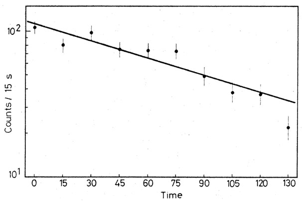
) comprises 68% of the Gaussian
distribution (see Fig. 5), there
is a 32% chance that a measurement will exceed these limits!