8. COMPARING THE DENSITY AND VELOCITY FIELDS

In this penultimate chapter, we bring the results of the previous chapters together with a discussion of analyses involving both the velocity and density fields. This can be done either by predicting the velocity field from redshift surveys using Eq. (150), and comparing with the observed velocities (Section 8.1), or predicting the density field from peculiar velocity surveys using Eq. (149), and comparing with the observed redshift surveys (Section 8.2).

8.1. Comparison via the Velocity Field

8.1.1. Cluster Infall Models

Much of the motivation for measuring the velocity field has been to compare it to models of what is expected given the density field. Our historical review of our gradual understanding of the nature of the large-scale flow field focussed on measurements of bulk flows, but in fact much of the motivation of the early work was for measurements of cluster infall. A spherically symmetric cluster embedded in a homogeneous medium induces a spherically symmetric radial velocity field. In linear theory, the cluster infall velocity is simply given by (Eq. 33) :

(212)

where r is the distance to the center of the cluster, and (r) is the mean overdensity within r. In fact, for a top-hat initial density perturbation (i.e., a spherically symmetric overdensity that is constant in amplitude out to some given radius), the evolution can be calculated exactly (Silk 1974 , 1977; Schechter 1980 ; Bertschinger 1985a b; Regös & Geller 1989) by writing the evolution of the perturbation and the background density as separate isotropic expanding or contracting bodies, and matching the boundary conditions at the edge of the tophat. For the case of an open universe with an initial mean tophat overdensity _i > 1 at a time when the Hubble constant was H_i and the density parameter was _i, the radial velocity field at time t is

(213)

where is defined implicitly by the equation:

(214)

Similar equations can be written down for a closed universe. Much of the early work on interpreting results of velocity fields concentrated on fitting these formulae to the infall around the Virgo cluster (Tonry & Davis 1981a b; Aaronson et al. 1982b ; Davis et al. 1982 ; Tully & Shaya 1984 ; Tammann & Sandage 1985 ; Gudehus 1989 ; cf., the review of Davis & Peebles 1983a). There has been a great deal of controversy in the literature about the amplitude of the cluster infall detected, with characteristic numbers at the Local Group ranging from 100 km s^-1 to 450 km s^-1 (Section 7.1); this, together with the uncertainty in the overdensity of the Virgo cluster itself in galaxies (Sandage, Tammann, & Yahil 1979 ; Davis et al. 1982 ; Strauss et al. 1992a), has meant that values of determined from Virgocentric infall have been equally uncertain. Bushouse et al. (1985) and Villumsen & Davis (1986) used N-body models to test the ability of this method to constrain ₀, and concluded that it works to the extent that one's peculiar velocity data surrounds 4 steradians of the cluster, otherwise, shear motions from more distant mass concentrations can strongly bias the results.

In the meantime, studies of the Virgo cluster have shown that the approximation of it as an isolated spherically symmetric cluster is less and less applicable. It has been known for years that it shows appreciable substructure on the sky; accurate distances to Virgo galaxies have shown that it probably has appreciable depth (at least in spiral galaxies), which may contribute to some of the controversy as to its distance, and the intrinsic scatter of the Tully-Fisher relation (Pierce & Tully 1988 ; Fukugita, Okamura, & Yasuda 1993). Moreover, the velocity field around it is affected by other, more distant, mass concentrations and voids; in particular, Lilje et al. (1986) demonstrated the presence of a tidal field in the Aaronson et al. (1982a) data from what we now interpret as the Great Attractor.

Spherically symmetric cluster infall models are starting to be applied to more distant clusters. Kaiser (1987) and Regös & Geller (1989) showed that cluster infall causes characteristic caustics in the redshift-space maps of galaxies around clusters, although the structure in the galaxy distribution in the field in which the cluster is embedded can make these caustics difficult to identify. Careful measurement of these caustics has the potential to yield the linear cluster infall velocity, which, together with the measured overdensity of galaxies in the clusters, will yield . However, it is not yet clear how practical this approach is given the complicated effects of intrinsic small-scale structure in the galaxy distribution outside the clusters themselves.

There have been a variety of attempts to go beyond the single cluster model for the velocity field by invoking two or more clusters (e.g., Faber & Burstein 1988 ; Han & Mould 1990 ; Rowan-Robinson et al. 1990), or even to fit the flow field around a void (Bothun et al. 1992). But given the availability of redshift surveys covering much of the sky, we can trace out the full density field at every point in space (at some modest smoothing length) in the local universe, and compare the resulting predicted velocity field (Section 5.9) with observations.

8.1.2. Unparameterized Velocity Field Models

In this section and the next, we describe the most direct comparisons between peculiar velocity and redshift surveys. Linear theory gives a relation between galaxy density and peculiar velocity (Eq. 33), which can be used to derive a velocity field from a redshift survey (Section 5.9). The resulting velocity field can be compared point-by-point with measured peculiar velocities in a Method I analysis (usually using the forward DI relations); the slope of the resulting scatter plot is thus in principle a measure of . This process is actually somewhat subtle: sampling the predicted peculiar velocity field at the measured distance of each galaxy gives biased results, due to the substantial errors in the distances. Rather, one should calculate the predicted peculiar velocities given the redshifts to each object, by inverting the predicted redshift-distance diagram along each line of sight. This is subject to the ambiguities of triple-valued zones (Fig. 11). Furthermore, because the self-consistent velocity field from the redshift survey predicts the peculiar velocity of the Local Group, this comparison is best made in the frame in which the Local Group is at rest. This will give different results from a comparison in the frame in which the CMB shows no dipole, because the IRAS velocity field does not exactly match the peculiar velocity of the Local Group (Section 5.7). Much of the early work in this field was done before a proper understanding of selection and Malmquist biases were at hand (Section 6.5), making these results somewhat suspect.

Strauss (1989) compared the IRAS 1.936 Jy predicted velocity field with the Mark II peculiar velocity data. A strong correlation between observed and peculiar velocities was seen, and the slope was consistent with = 0.8. Similar results were found by minimizing the scatter in the inverse Tully-Fisher relation for the Aaronson et al. (1982a) data in a Method II analysis. However, the error in the derived was not properly quantified; nor for that matter was it demonstrated that the scatter was consistent with the observational errors.

Kaiser et al. (1991) used a Method I approach to compare the velocity field from the QDOT redshift survey with the Mark II data. The QDOT density field (and therefore predicted velocity field) was corrected for redshift space distortions not by iterations, as in Section 5.9, but rather by applying a correction to the smoothed density field at each point taken from Kaiser (1987) (cf, Eq. 91). The resulting predicted peculiar velocity field was compared to the Mark II data, binned on the same grid used to define the density field; least-squares fits yielded a slope = 0.86 ± 0.14.

A similar approach was taken by Hudson (1994b) who used the density field of optically selected galaxies to obtain a predicted peculiar velocity field to compare with the Mark II data. He used the techniques of Hudson (1994a) to correct the data for inhomogeneous Malmquist bias, assuming the galaxies for which peculiar velocities were measured to be drawn from the same density distribution as in his maps. He also included in his models a bulk flow from scales beyond those surveyed. He concluded from his peculiar velocity scatter plots that = 0.50 ± 0.06, with an additional bulk flow of 405 km s^-1 towards l = 292°, b = + 7°. However, this derived bulk flow is almost in the Galactic plane, in the direction of the Great Attractor, and thus may be due to overdensities not surveyed by Hudson's sample. On the other hand, this bulk flow is roughly consistent with that observed from the Mark III data, so it may indeed represent flows on scales larger than his sample.

Shaya, Tully, & Pierce (1992) also compared peculiar velocities (in this case, from a combination of the Aaronson et al. (1982a) data and their own TF data; Tully, Shaya, & Pierce 1992) with a redshift survey, namely the catalog of galaxies within 3000 km s^-1 compiled by Tully (1987b) . They used luminosity rather than number weighting, and carried out an elaborate analysis which includes components to the density field clustered on a variety of length scales. They concluded that ₀ associated with galaxies is only 0.1, clustered on 1 h^-1 Mpc scales. However, their modeling of the effects of mass concentrations in the Zone of Avoidance, and beyond 3000 km s^-1, is simplistic, and their resulting predicted peculiar velocity field only bears qualitative resemblance to that measured. A more recent analysis is presented by Shaya, Peebles, & Tully (1994) , using Peebles' (1989) variational technique to extend the linear theory relation between the density and velocity fields. They conclude that _optical < 0.4, but emphasize that their analysis is still in progress, and awaits improved Tully-Fisher data.

Roth (1993; 1994) carried out a Tully-Fisher survey in the I band of 91 galaxies selected from a volume-limited subset of galaxies within 4000 km s^-1 from the 1.936 Jy IRAS redshift survey, and minimized the scatter of the forward Tully-Fisher relation as a function of in the IRAS velocity field model, using a Method II approach. Extensive Monte-Carlo simulations demonstrated that this method gives an unbiased estimate of ; he found ~ 0.6. Unfortunately, systematic errors in the line-width data, and the dominance of the triple-valued zone around the Virgo cluster (which is prominent in the sample) mean that the systematic errors associated with this result are large. Schlegel (1995) is extending the survey to contain ~ 250 galaxies with accurately measured line widths from H rotation curves, and with more uniform sky coverage; this dataset promises to give tighter constraints on .

Finally, Nusser & Davis (1994a) compared the predicted dipole moment of their multipole expansion of the IRAS velocity and density field (cf., Eq. 145) with that measured from the POTENT map. They show that the dipole of a shell as measured in the Local Group frame depends only on the density field interior to that shell, making this a semi-local comparison. They conclude = 0.6 ± 0.2, although the error was estimated by eye from their plots. This is a promising way to proceed, especially with their more sophisticated technique for determining the multipole moments of the measured velocity field (Section 7.5.4).

8.1.3. Method II ⁺

Common to the handful of Method II velocity comparisons discussed above is the assumption of a unique redshift-distance mapping, as required in a Method II analysis (Section 6.4.3). In the real world, however, a distance cannot be unambiguously assigned from an observed redshift - even when the peculiar velocity model is "correct." In what follows, we explain why this is so, and describe a maximum likelihood method to overcome the problems that result.

One can distinguish two contributions to a galaxy's peculiar velocity. The first is what is usually meant by the peculiar velocity "field." It has a coherence length of a few Mpc or greater, is due to perturbations in the linear or quasi-linear regime, and is predictable from an analysis of density fluctuations. The second is what is loosely referred to as velocity "noise." It has zero coherence length, arises from strongly nonlinear processes, and is unpredictable except in a statistical sense. We label the coherent part v(r), and describe the random part in terms of an rms radial velocity dispersion _v. Each can separately invalidate the assumption of a unique redshift-distance mapping, as follows:

1. Method II assumes that the distance r to a galaxy is the "crossing point" in the redshift-distance diagram, given implicitly by

   (215)

   (cf. Section 6.4.3). There is, however, no guarantee that this equation will have only one solution. When line of sight gradients in v(r) are of order unity, there can be three or more crossing points for given cz. Such regions are generically called "triple-valued zones" (cf., Fig. 11).

2. Even if Eq. 215 has a unique solution r, this solution will differ from the true distance because of velocity noise. In essence, cz is a random realization of the "redshift field" r + . v(r), and only defines the crossing point to accuracy ~ _v.

The situations just described are summarized in Fig. 11, which shows a triple-valued zone around the Virgo cluster. The inherent uncertainty due to velocity noise is indicated with the scatter of points.

Because of these effects, Method II is subject to biases over and above selection bias (Section 6.4). Willick et al. (1995d) have developed a modified form of Method II which neutralizes these biases by explicitly allowing for non-uniqueness in the redshift-distance mapping. The basic idea is to derive correct probability distributions of observable quantities, taking into account the complexities of the redshift-distance relation, and then to maximize likelihood over the entire data set. This approach shares features of both Methods I and II (Section 6.4.3), but is closer in spirit to the latter, and will accordingly be called "Method II⁺" in what follows.

We assume the goal is to fit a model peculiar velocity field v(r; a), where a is a vector of free parameters, and adopt the useful abbreviation

(216)

for its radial component. The central element of Method II⁺ is a description of the redshift-distance relation in terms of a Gaussian probability distribution:

(217)

A related probability function is given as a function of r in the lower half of Fig. 11 (that curve shows the probability distribution in Eq. (144), which differs from P(cz| r) by the additional factors of n(r)r² (4 r²f_min)). Three subtleties of Eq. (217) deserve mention. First, _v is not merely the true velocity noise, whose value is thought to be ~ 150 km s^-1 (e.g., Groth et al. 1989), but rather its convolution with two additional effects: redshift measurement errors and velocity model errors. The former are small (typically ~ 50 km s^-1) but not entirely negligible. The latter, which reflect the finite accuracy of our predictions, can be estimated from N-body simulations (e.g., Fisher et al. 1994d) and are of order 200 km s^-1. Second, _v is not necessarily constant; both the true velocity noise and model errors are larger in dense regions. Third, whereas true velocity noise is incoherent, model prediction errors are not. Contributions to v(r) arising on scales too small to be included in the model, but which unlike true noise have spatial coherence, manifest themselves as coherent prediction errors. In what follows, we will neglect these subtleties and treat _v as a spatial constant of order 200 km s^-1 whose value may be held fixed or treated as a free parameter in the likelihood analysis.

We quantified Method II selection bias (Section 6.5) based on the probability distribution P(m, , r), arguing that we could in effect treat redshift as distance. Using Eq. (217), we may now write down the joint distribution of the TF observables, distance, and redshift:

(218)

where we have assumed that the TF observables and redshift couple only via their mutual dependence on true distance. The observables in a redshift-distance sample are m, , and cz. Their distribution is obtained by integration:

(219)

Eq. (219) gives the likelihood of a data point in a redshift-distance sample, valid for arbitrary v(r;a) and _v. Method II⁺ consists of maximizing the product of the likelihood (Eq. 219) over the peculiar velocity sample, with respect to the parameters of the velocity field model, the parameters of the TF relation (including its scatter), and _v.

The overall likelihood depends on TF probability evaluated not only at the crossing point(s), but over a range of distances roughly characterized by

(220)

This likelihood will differ from its Method II counterpart to the extent that the length scale on which P(m,, r) varies is comparable to or smaller than the interval defined by Eq. (220). The former scale is given by ~ d, where is the TF fractional distance error and d = 10^{0.2[m - M()]} is the inferred distance (Section 6.5.2). For galaxies beyond 3000 km s^-1, d 600 km s^-1. This is considerably larger than the range given by Eq. (220) for typical _v, outside triple valued or flat zones. In these circumstances Methods II and II⁺ differ little. Indeed, it is easy to see that--again away from triple-valued or flat zones - Method II⁺ reduces exactly to Method II (Eq. 165) in the limit _v -> 0. However, Method II⁺ represents a substantial correction to classical Method II at small (d 2000 km s^-1) distances, in triple-valued or flat zones, or when _v becomes anomalously large. Method II⁺ is therefore necessary for rigorous analysis of the very local universe and, in particular, of the Local Supercluster region, where small distances and triple-valuedness are often combined.

Application of Method II⁺ requires two additional steps. First, one must decide whether to use the forward or inverse form of the TF relation, and thus whether Eq. (171) or Eq. (188) is used for P(m,, r) in Eq. (219). As in Method II (Section 6.4), the inverse method is advantageous when sample selection is independent of velocity width ⁽³⁵⁾ , though with Method II⁺ this choice introduces a new uncertainty discussed below. Second, one does not apply Eq. (219) directly, but instead derives from it suitable conditional probabilities: P(m|, cz) in the forward case, P( | m, cz) in the inverse. These are obtained from Eq. (219) as follows:

(221)

and

(222)

where we have restored the compact notation P(cz| r) (Eq. 217), reversed the order of integration in the denominators, and allowed for an explicit r-dependence of sample selection (which in fact exists for some of the Mark III samples; cf. Section 6.5.3). The integrals over m and in the denominators of Eqs. (221) and (222) can be done analytically for simple forms of S (Willick 1994), so two-dimensional integrations are not required. The chief advantage of conditional probabilities is that they are less sensitive than P(m,, cz) to the precision with which the number density n(r) is modeled. As n(r) appears in both numerator and denominator, it only weakly affects the conditional distributions provided it varies slowly compared with P(cz| r) or the TF probability term, as will generally be the case. This is important, since it is the accuracy of our velocity model, not our density model, with which we are mainly concerned. Still, Method II⁺ (unlike Method II) does require a density model, and in that sense resembles a Method I analysis. Finally, note that the velocity width distribution function () (Section 6.5) strictly cancels out of P(m|, cz), while the luminosity function (M) (Section 6.5.4) does not cancel out of P( | m, cz) (although the results are insensitive to the luminosity function, as it again appears in numerator and denominator).

Willick et al. (1995d) used Method II⁺ to analyze data from the Mark III peculiar velocity catalog (Section 7.2). They limited their analysis to the 900 galaxies in the TF samples of Mathewson et al. (1992b) and Aaronson et al. (1982b) , which densely sample the local region, and to redshifts 3500 km s^-1. The forward method (Eq. 221) was used, and the TF parameters for each sample (slope, zeropoint, and scatter) were allowed to vary in the search for maximum likelihood, rather than fixing them at their values determined in the Mark III analysis (Section 7.2).

The IRAS 1.2 Jy predicted peculiar velocity field was taken as the model to be fitted to the data. To first order this model velocity field depends only on , although the analysis was carried out for two different smoothing lengths, and with and without nonlinear effects included. Using the IRAS galaxy density field for the quantity n(r) that appears in Eqs. (221) and (222) assumes that IRAS galaxies are distributed like the Mark III sample objects. This assumption may not be correct in detail but is expected to have a minimal effect on our conditional analysis. The forward Method II⁺ analysis was carried out in terms of a quantity defined by

(223)

where the sum runs over all galaxies used in the comparison. An analogous statistic using the inverse relation is discussed by Willick et al. and gives consistent results.

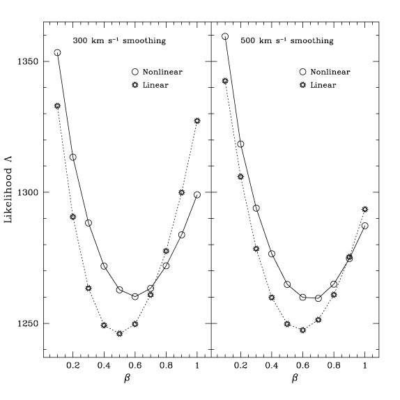
Figure 18. Likelihood plotted as a function of for four realizations of the IRAS predicted peculiar velocity and density fields. Likelihoods have been computed using a Method II+ comparison with a subset of the Mark III peculiar velocity catalog (see text for details). The left hand panel depicts results in which a 300 km s-1 smoothing length was used in the IRAS velocity and density field reconstruction; a 500 km s-1 smoothing length was used in the right hand panel. Each panel shows the results for linear (dotted line) and nonlinear (solid line) predictions. The latter were obtained by holding the bias factor fixed at b = 1.

We summarize these results in Fig. 18, which shows vs. curves for four realizations of the IRAS fields: 300 and 500 km s^-1 gaussian smoothing lengths, each with and without nonlinear corrections, following Nusser et al. (1991) , and setting b = 1. The "best" values of occur at the minima of the curves; they range from 0.48 for 300 km s^-1 smoothing linear to 0.65 for 500 km s^-1 smoothing nonlinear. The statistical error at 95% confidence level associated with these numbers is ~ 0.15, as determined by deviations of the likelihood function from its minimum. Note that there are systematic effects acting as well: a larger smoothing length leads to a larger , and nonlinear corrections yield larger for a given smoothing length. These results are to be expected: both increasing the smoothing scale and making nonlinear corrections decrease the amplitude of predicted peculiar velocities, and thus are qualitatively similar to decreasing . For the nonlinear fields, the predicted velocities now depend separately on ₀ and b; the curves here were obtained for the case b = 1, i.e., = ₀^0.6.

Which of the four IRAS predicted velocity fields shown should ideally be used in estimating ? In Method II⁺ we are comparing the predicted velocity field with unsmoothed data. The field obtained from 300 km s^-1 smoothing thus gives rise to the most valid comparison here. At smaller smoothing lengths the nonlinear corrections cease to be valid. Nonlinear effects must be present, as the overdensities at 300 km s^-1 smoothing can be considerably in excess of unity. However, Fig. 18 shows that the nonlinear curve has formally smaller likelihood than the linear curve. The reason for this is not well understood at present. A compromise value is 0.55, roughly midway between the linear and nonlinear minima. It is not clear how to combine the systematic and statistical errors we have identified; for now we conservatively put the 95% confidence level at ± 0.25.

As mentioned above the value of the rms velocity noise _v was treated as a free parameter, its final value determined by maximizing likelihood for each . Willick et al. found that _v 150-160 km s^-1 for the likelihood-maximizing values of . This value is remarkably small, in view of the fact that the IRAS predictions themselves are thought to have rms errors of 100-200 km s^-1, as discussed above; the implication would appear to be that the true noise is 100 km s^-1. It is unlikely that the velocity field is in reality that cold. It is likely instead that by neglecting correlated model prediction errors (see above), the likelihood analysis ends up underestimating _v. Future implementations of both Method II⁺ (and Method II, which similarly assumes uncorrelated residuals) will need to address this issue.

8.2. Comparison via the Density Field

The reconstruction of the mass density field using the POTENT method begs a comparison with the galaxy density field as observed in redshift surveys. Indeed, to the extent that the two fields are proportional to one another, their ratio gives a measure of via Eq. (149). Dekel et al. (1993) carried out this comparison, using the Mark II POTENT maps of Bertschinger et al. (1990) and the IRAS 1.936 Jy redshift survey. The first, and most striking result from this comparison, is that the POTENT and IRAS density field show qualitative agreement. Given the noise and sparseness in the peculiar velocity data, the POTENT map has much greater noise than does the IRAS map, and therefore the region in which the comparison of the two can be made is limited. Nevertheless, both show the Great Attractor and the void in front of the Perseus-Pisces supercluster. With 1200 km s^-1 Gaussian smoothing, there are ~ 10 independent volumes within which the comparison of the two density fields can be made. A scatter plot of the two shows a strong correlation. In the absence of biases, the slope of the regression would be an estimate of . However, as discussed in Section 7.5, the POTENT density field is subject to a number of biases. The most severe of these in this context is Sampling Gradient bias, with inhomogeneous Malmquist bias taking a close second. One can quantify the first by sampling the IRAS predicted velocity field at the positions of the Mark II galaxies, and running the results through the POTENT machinery; comparing the resulting density field to the input density field yields a regression slope of 0.65, substantially different from unity. Given this fact, Dekel et al. used an elaborate maximum likelihood technique to quantify the agreement between the POTENT and IRAS density fields. For a given value of (actually given values of ₀ and b; Eq. (209) rather than Eq. (149) is used throughout), they create mock Mark II datasets given the IRAS predicted peculiar velocity field (via the method described in Section 5.9), noise is added, and the results are fed into POTENT. Note that these simulations suffer from sampling gradient bias exactly as does the real POTENT data. The slope and scatter of the regression between the original IRAS map and the mock POTENT map are recorded, and the two-dimensional distribution of these two quantities is calculated for 100 such realizations. Elliptical fits to this distribution allows them to calculate the probability that the observed slope and scatter of the regression is consistent with the model assumed (i.e., the IRAS predicted peculiar velocity field for the given values of ₀ and b are consistent with the observed peculiar velocity field, given the errors). This process is then repeated for a grid of values of ₀ and b.

The conclusions from this work are as follows:

1. There exist values of ₀ and b for which the likelihood that the model is is consistent with the data is high. That is, the observed scatter is consistent with the assumed errors and the assumption that IRAS galaxies are at least a biased tracer of the density field that gives rise to the observed peculiar velocities.
2. The tightest constraint is on , for which the likelihood curve gives = 1.28_-0.59^+0.75 at 95% confidence.
3. Not surprisingly, the constraints on ₀ and b separately are quite a bit weaker. Indeed, the likelihood contour levels do not close at large ₀ for a given , meaning that the data are consistent with purely linear theory in which no second-order effects exist. The data are inconsistent with highly non-linear conditions (i.e., very small ₀ for a given ), but this is the regime in which the non-linear approximation used starts to break down anyway.

May we then conclude that the gravitational instability picture has been proven? After all, we have seen consistency in the data with one of its strongest predictions, namely Eq. (30). However, as Babul et al. (1994) emphasize, Eq. (30) can be derived directly from the first of Eqs. (21), the continuity equation alone; only the constant of proportionality comes from gravity. Indeed, and ^. v are proportional for any model in which galaxies are a linearly biased tracer of the mass, and for which the time-averaged acceleration is proportional to the final acceleration. They show analytically and with the aid of simulations that a range of models with non-gravitational forces exhibit correlations between and ^. v at least as strong as that seen in the POTENT-IRAS comparison. Thus a proof of the gravitational instability picture will require ruling out these alternative models by other means.

Work is in progress as this review is being written, to update the POTENT results using the Mark III peculiar velocity compilation. The Mark III data have been corrected for inhomogeneous Malmquist bias, assuming that the IRAS density field is that of the galaxies of the Mark III sample. More importantly, however, the systematic errors in the overlap between datasets have been minimized, and the volume surveyed well with the Mark III data is such that the IRAS-POTENT comparison can be done over four times as many data points as before. In addition, the more complete sampling means that the sampling gradient bias is smaller than with the Mark II data, by roughly a factor of two in the mean. The left-hand panel of Fig. 19 shows a preliminary version of the POTENT density field in the Supergalactic plane using 1200 km s^-1 Gaussian smoothing, taken from Fig. 17. The right hand panel shows the density field of the IRAS 1.2 Jy survey at the same smoothing. The qualitative agreement is remarkable. In the Supergalactic plane, both maps show the Great Attractor, the Perseus-Pisces Supercluster, the Coma-A1367 Supercluster, as well as voids between Coma and Perseus, and South of the Great Attractor (the Sculptor Void). Work is ongoing to quantify the differences between the two maps, and to put exact error bars on the derived .

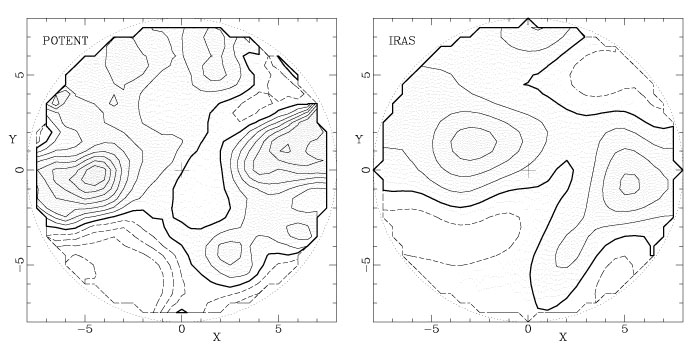
Figure 19. The left panel is the POTENT density field . v in the Supergalactic plane from the Mark III peculiar velocity data. The right panel is the independently determined density field of IRAS galaxies. The smoothing in both panels is 1200 km s-1. The axes are labeled in 1000 km s-1. The Local Group sits at the center of each panel.

Hudson et al. (1995) have carried out a comparison of the Mark III POTENT results with the optical galaxy density field of Hudson (1993a, b). They also find good agreement. between the two density fields; a less elaborate analysis than that of Dekel et al. (1993) shows = 0.74 ± 0.13.

³⁵ In principle, Method II⁺ rigorously incorporates selection effects into either the forward or inverse formalism. However, with real data characterization of sample selection is often subject to uncertainty (Willick et al. 1995a b). Its relatively smaller susceptibility to selection bias thus remains a virtue of the inverse approach. Back.