


In this brief concluding chapter, we summarize what it is that has been learned from redshift and peculiar velocity surveys, and put the results into the context of the larger field of observational cosmology.
9.1. The Initial Power Spectrum
We have put constraints on the power spectrum directly from measurements of the distribution of galaxies (Section 5.3). The fact that power spectra derived from redshift surveys in different areas of the sky, using different samples, agree, implies that it is meaningful to define a power spectrum in the first place. That is, we do not live in a simple fractal universe, in which a mean density depends on the scale on which it is measured. Moreover, our samples are starting to become big enough that our statistical measures are not completely dominated by sampling fluctuations, at least for measures probing relatively small scales (50 h-1 Mpc and smaller). This is not to say that improvements in the statistical errors in the power spectrum on these scales are not needed!
The redshift survey data strongly rule out the standard CDM model, and
are fit much better by a
 = 0.20 - 0.30 model
(Fig. 9). This is in accord with
analyses of the
small-scale velocity dispersion of galaxies, their large-scale angular
clustering, observations of bulk flows on large scales, as well as
constraints from the CMB fluctuations
(Efstathiou et
al. 1992;
Kamionkowski &
Spergel 1994
; Kamionkowski, Spergel,
& Sugiyama 1994
), the distribution and mass spectrum of clusters
(Bahcall & Cen 1992
; 1993),
and a host of other constraints. Unfortunately, we cannot
conclude from this that the dark matter problem is solved. A number of
the different suggested power spectra are degenerate over the scales
probed by redshift surveys, with very different implications for the
nature of the dark matter (compare the range of
Fig. 9
to that of Fig. 2). In particular,
the data we have
presented are also consistent with the Mixed Dark Matter model and the
Tilted Cold Dark Matter model, which are two of the more popular
models being discussed.
= 0.20 - 0.30 model
(Fig. 9). This is in accord with
analyses of the
small-scale velocity dispersion of galaxies, their large-scale angular
clustering, observations of bulk flows on large scales, as well as
constraints from the CMB fluctuations
(Efstathiou et
al. 1992;
Kamionkowski &
Spergel 1994
; Kamionkowski, Spergel,
& Sugiyama 1994
), the distribution and mass spectrum of clusters
(Bahcall & Cen 1992
; 1993),
and a host of other constraints. Unfortunately, we cannot
conclude from this that the dark matter problem is solved. A number of
the different suggested power spectra are degenerate over the scales
probed by redshift surveys, with very different implications for the
nature of the dark matter (compare the range of
Fig. 9
to that of Fig. 2). In particular,
the data we have
presented are also consistent with the Mixed Dark Matter model and the
Tilted Cold Dark Matter model, which are two of the more popular
models being discussed.
The Mixed Dark Matter model has a long history, starting with the idea that adiabatic damping of the power spectrum on small scales by baryons will cause a turn-down in the power spectrum (Silk 1968 ; Dekel 1981); its recent incarnation is in terms of a mix of hot and cold dark matter (Schaefer, Shafi, & Stecker 1989 ; Schaefer & Shafi 1992 ; Taylor & Rowan-Robinson 1992 ; Davis, Summers, & Schlegel 1992 ; Klypin et al. 1993). In particular, the hot dark matter suppresses the power spectrum on small scales, decreasing the small-scale velocity dispersion relative to standard CDM, and increasing the amount of large-scale power for a given normalization on small scales. However, the model perhaps suppresses small-scale power overly much: galaxies cannot form on these small scales until very late, which is difficult to reconcile with observations of galaxies and quasars at very high redshifts (Cen & Ostriker 1994 ; cf., Efstathiou & Rees 1988 for a similar critique of standard CDM).
The tilted CDM model was suggested simultaneously by a number of workers (Cen et al. 1992 ; Lidsey & Coles 1992 ; Lucchin, Matarrese & Mollerach 1992; Liddle, Lyth & Sutherland 1992; Adams et al. 1993 ; Cen & Ostriker 1993). It also increases the amount of power on large scales relative to small, in this case by changing the slope of the primordial power spectrum. However, Muciaccia et al. (1993) showed that standard CDM is preferred over tilted models when velocity field data and CMB fluctuations are taken into account as well.
There are a number of further constraints on the power spectrum, some
of which we've only touched upon on this review. The most important of
these is the fluctuations in the CMB. On the largest scales, the
fluctuations as detected by COBE appear to be consistent with a
primordial power spectrum of index n = 1 (the inflationary
prediction)
(Górski et
al. 1994),
with an amplitude that matches well that predicted from the
= 0.2 CDM model
(Fig. 9). Observations of the CMB
fluctuations on
sub-COBE scales (a few degrees) are just beginning to yield
reproducible results; because more than the Sachs-Wolfe effect is
operating on these smaller scales, these data can potentially yield
information on  0,
the density parameter in baryons, as well as the power spectrum
(Hu & Sugiyama
1995).
In addition, these probe
scales now being reached by the largest peculiar velocity and redshift
surveys, spanning much of the gap seen in
Fig. 2. In
this regard, the bulk flow results of
Lauer & Postman
(1994)
(Section 7.1.4) remain unexplained in
the context of
models for large-scale structure. It is vitally important that this
result be checked, as a number of workers are now doing
(Section 9.7). The comparison between large-scale
flows and
CMB fluctuations has the potential to check gravitational instability
theory directly, independent of the power spectrum
(Juszkiewicz,
Górski, & Silk 1987
;
Tegmark, Bunn & Hu
1994).
0,
the density parameter in baryons, as well as the power spectrum
(Hu & Sugiyama
1995).
In addition, these probe
scales now being reached by the largest peculiar velocity and redshift
surveys, spanning much of the gap seen in
Fig. 2. In
this regard, the bulk flow results of
Lauer & Postman
(1994)
(Section 7.1.4) remain unexplained in
the context of
models for large-scale structure. It is vitally important that this
result be checked, as a number of workers are now doing
(Section 9.7). The comparison between large-scale
flows and
CMB fluctuations has the potential to check gravitational instability
theory directly, independent of the power spectrum
(Juszkiewicz,
Górski, & Silk 1987
;
Tegmark, Bunn & Hu
1994).
Constraints can be put on the power spectrum from observations of
galaxies at high redshift. The amount of small-scale power determines
at what epoch galaxies will form; measures of the age of galaxies and
their evolution thus tell us something about the power
spectrum. Balancing the need for enough small-scale power to allow
galaxies to form early, as seems to be required by observations of
high-redshift galaxies and quasars, against the requirement of not too
much small-scale power, in order to restrict the small-scale velocity
dispersion (Section 5.2.1) has not yet
been self-consistently done for any model.
Similarly, observations of clusters of galaxies and their
evolution also have the power to constrain cosmological models (eg.,
Peebles, Daly, &
Juszkiewicz 1989).
Finally, detection of the
evolution of clustering in the universe would be a tremendously
important observation. In an open universe, clustering ceases to grow when
deviates significantly from
unity (Section 2.2);
unambiguous detection of this effect would be a sensitive measure of
0.
Perhaps the most dramatic constraint one could imagine on the power spectrum would be the laboratory detection of dark matter (Primack et al. 1988). It would be a tremendous triumph of our theoretical framework if a dark matter particle were discovered with properties consistent with the best-fit power spectrum from astronomical data. The HDM model has been out of favor for some time, given its unphysically late formation epoch for galaxies (e.g., White, Frenk, & Davis 1983), but if a definite non-zero mass for the muon neutrino were measured appropriate to close the universe, HDM models would certainly enjoy a resurgence of popularity!
9.2. The Distribution Function of the Initial Fluctuations
All the tests we have described for the random-phase hypothesis have yielded positive results; there is no direct evidence for non-Gaussian fluctuations in the initial density field. Perhaps the strongest such claim comes from the direct measure of the distribution function of initial fluctuations as found by the time machine of Nusser & Dekel (1993) . Similar conclusions are found in analyses of the COBE CMB fluctuations (e.g., Hinshaw et al. 1994). However, as we emphasized in Section 5.4, this by no means allows us to conclude that all non-Gaussian models are dead. Each of the tests described in Section 5.4 refer to a specific smoothing scale, and a model that is non-Gaussian on a given scale need not be so on another. What is needed is a systematic test of each non-Gaussian model proposed against the various observational constraints. This has been done to a certain extent for models of cosmic strings (Bennett, Stebbins, & Bouchet 1992) and texture models (Pen, Spergel, & Turok 1994), mostly in the context of non-Gaussian signatures in CMB fluctuations.
9.3. The Gravitational Instability Paradigm
The results we have presented here are all consistent with the gravitational instability picture. In particular, we have seen that there exist physically plausible power spectra which can simultaneously match the observed large-scale distribution of galaxies, large-scale flows, and the CMB fluctuations (36) . When redshift surveys began to reveal extensive structures such as giant voids and the Great Wall, many questioned whether this could be explained in the context of gravitational instability theory. However, simulations by Weinberg & Gunn (1990) , and Park (1990) , as well as arguments based on the Zel'dovich approximation (Shandarin & Zel'dovich 1989), showed that these structures were not unexpected given gravitational instability and plausible models for the power spectrum.
The most direct test of gravitational instability comes from the comparison of peculiar velocity and redshift surveys. Dekel et al. (1993) in particular claim that the Mark II peculiar velocity data are consistent with the velocity field predicted from the distribution of IRAS galaxies, and gravitational instability theory. However, this is not a proof; Babul et al. (1994) demonstrate models with velocities due to non-gravitational forces (in particular, large-scale explosion models) that the Dekel et al. tests would not rule out.
We have not discussed features of the velocity field on small scales, smaller than are resolved by the POTENT-IRAS comparison, with its 1200 km s-1 Gaussian smoothing. Burstein (1990) presents evidence that the very local velocity field, as measured with the Aaronson et al. (1982a) TF data, differ qualitatively from the IRAS predictions, a conclusion that continues to hold with the Tormen & Burstein (1995) reanalysis of the Aaronson et al. data. Similarly, the complete lack of an infall signature in the spiral galaxies around the Coma cluster found by Bernstein et al. (1994) is worrisome, and remains unexplained. Understanding these results remains a task for the future.
Gravitational instability theory has given us a tool to measure the
cosmological density parameter, by comparing peculiar velocities with
the density distribution (Eq. 30), although in most
applications, galaxy biasing means that we constrain only

 00.6 /
b. In Table 3, we summarize the various
constraints on 0
that we have discussed in this review.
00.6 /
b. In Table 3, we summarize the various
constraints on 0
that we have discussed in this review.

Is there some consensus in the literature as to the value of
?
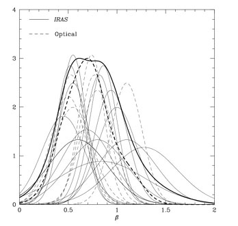
One way to assess this, at least qualitatively, is to plot each of the
determinations in Table 3 as a series of
Gaussians of unit integral,
with means and standard deviations given by the numbers in the table.
For simplicity, asymmetric error bars have been symmetrized, and
those determinations without quoted error bars are not included.
Determinations based on IRAS and optical samples are plotted with
different symbol types. We now simply add the Gaussians together, to
yield the two heavy curves in the plots. Note that this procedure
tends to give lower weight to those determinations with more realistic
(i.e., larger) error bars. No attempt has been made to assess the
relative quality of these different determinations. Note also that
because many of these determinations are from common datasets, they
are not independent. Thus this form of qualitative summary gives an
unprejudiced view of literature of determinations of
from redshift
and peculiar velocity surveys. The heavy curves have a mean of 0.78
and standard deviation of 0.33 (IRAS) and a mean of 0.71 and
standard
deviation of 0.25 (optical). These values are actually in quite close
agreement, although that seems more coincidental than anything else,
given the large spread of individual determinations.
The community is clearly not quite ready to settle on a single value
for for the IRAS
galaxies. The determinations range from 0.45
(Fisher et al. 1994b)
to 1.28
(Dekel et al. 1993
,
although the
latter is likely to come down slightly with the Mark III data; Dekel,
private communication). This is reflected in the large standard
deviation, larger than any individual determination, and the flat top
to the heavy curve in Fig. 20 . The optical
shows a smaller spread,
perhaps simply because there are fewer
individual determinations of it. The odd man out is the determination
of 0 by
Shaya et al. (1994),
although their determination is
heavily affected by their modeling of the background density within
3000
km s-1 and the density field beyond there. Moreover, their work
remains in flux (compare with
Shaya et al. 1992)
and it is not clear where their final results will lie.
|
Figure 20. The distribution of
determinations of |
Most of the references in Table 3 are very recent, and we have not
done a thorough job of reviewing the earlier literature, especially on
Virgocentric infall. However, the common impression that estimates of
0 have taken a
dramatic upturn in recent years is wrong.
Davis et al. (1980)
used observations of Virgocentric flow to find
= 0.6 ± 0.1, in good
agreement with the values for optical
galaxies here. The value from the Cosmic Virial Theorem from
Davis & Peebles
(1983b)
is difficult to interpret in terms of a biasing model,
but corresponds to
= 0.4 for an unbiased model.
9.5. The Relative Distribution of Galaxies and Mass
We have very few handles on the biasing parameter independent of
. One approach has been to
assume a model for the power
spectrum, normalize it to the COBE fluctuations, and then compare the
results predicted for the galaxy fluctuations at 8 h-1
Mpc with
observations. This approach is by definition model-dependent; for
standard CDM, one finds that optical galaxies are unbiased and that
IRAS galaxies are anti-biased, while a model like
= 0.2 CDM
gives a normalization that leaves the IRAS galaxies unbiased.
Alternatively, one can constrain biasing by looking for non-linear
effects to break the degeneracy between
0 and b. The
skewness is one such effect. Fry & Gaztañaga
(1993;
1994)
and
Frieman &
Gaztañaga (1994)
claim that the beautiful agreement
between the measured higher-order moments of the APM counts-in-cells
with that predicted given the power spectrum, implies that biasing of
optical galaxies is very weak, and to the extent that there is
biasing, that it is local.
Dekel et al. (1993)
attempted to look for
non-linear effects in the IRAS-POTENT comparison; they could only
show that the data are inconsistent with very strong non-linearities,
thereby ruling out very small values of b.
Finally, one can look for relative biasing of different types of galaxies, as we described in Section 5.10. The effects are subtle: outside of clusters, there are no two populations of galaxies known that have qualitatively different large-scale distributions. The lack of such effects have motivated several workers (Valls-Gabaud et al. 1989; Peebles 1993) to argue that biasing cannot be acting at all. But differential effects are seen between galaxies of different luminosities and morphological types. It is time for a detailed comparison of these observed effects with hydrodynamic simulations, in order to see what constraints these put on general biasing schemes.
In any case, the consensus of the community is that biasing is
relatively weak; few authors are arguing for b > 1.5 these
days. This is quite a contrast to a decade ago, when the idea of
biasing was first introduced; values of b = 2.5 or higher were
popular (e.g.,
Davis et al. 1985).
Thus we conclude that
5/3 <
0 <
25/3; the results
of Table 3 are still consistent
with values in the range
0 = 0.3 to
0 = 1. It has
been quite popular in recent years to argue for the lower value, given
the coincidence with the value of
0 needed to match the
= 0.25 value preferred by
the power spectrum
(Coles & Ellis
1994).
9.6. Is the Big Bang Model Right?
One tests the Big Bang model with redshift and peculiar velocity data
only to the extent that they give results which can be fit into our
grander picture of the evolution of the universe, with input from all
the subjects we did not discuss: observations of distant galaxies and
quasars, measurements of individual galaxy properties, abundances of
the light elements, and so on. We should point out one serious problem
which we see on the horizon. The data we have discussed point towards
a value of 0
close to unity, implying an age of the universe given roughly by
t0 = 2/3 H0-1
(Eq. 17). With recent
determinations of the Hubble Constant of the order of 80
km s-1 Mpc-1
(Jacoby et al. 1992
;
Pierce et al. 1994
;
Freedman et al. 1994),
this gives an age of 8 billion years, less than half the
currently accepted ages of the oldest globular clusters (e.g.,
Chaboyer, Sarajedini,
& Demarque 1992).
Note that this would be a problem even if
0 -> 0, for which
t0 = 1 / H0 = 12 billion years. We
may find ourselves invoking theoretically awkward models in which
0


 1. In
any case, the next few years should be very exciting, as we come to
grips with this rather basic problem.
1. In
any case, the next few years should be very exciting, as we come to
grips with this rather basic problem.
We conclude this review with a quick discussion of the various on-going and planned redshift surveys and peculiar velocity surveys of which we are aware. As these become available, we can look forward to applying the statistics developed so far to vastly superior datasets; moreover, these will allow us to do analyses of much more subtle statistics.
There are a number of large-scale peculiar velocity surveys in progress. Giovanelli, Haynes, and collaborators are doing a Tully-Fisher survey of Sc I galaxies from the Northern sky drawn from the UGC catalog, together with calibrating galaxies drawn from a number of clusters. They have data for roughly 800 galaxies. In the meantime, Mathewson & Ford (1994) have extended their Tully-Fisher survey in the Southern Hemisphere to smaller diameters, as reported in Section 7.1.3; their sample now includes a total of 2473 galaxies.
At higher redshift, a team of eight astronomers started by three of
the original 7 Samurai (Burstein, Davies, and Wegner), has extended
the 7 Samurai
Dn- survey
of elliptical galaxies to a
further ~ 500 galaxies in clusters at redshifts
~ 10, 000 km s-1
(Colless et al. 1993).
survey
of elliptical galaxies to a
further ~ 500 galaxies in clusters at redshifts
~ 10, 000 km s-1
(Colless et al. 1993).
Several groups are attempting to check the large-scale bulk flow
measured by
Lauer & Postman
(1994) .
The same authors, in
collaboration with Strauss, are in the process of extending the survey
to include the BCG's of all Abell clusters to z = 0.08, a total of
over 600 clusters. They expect to complete the gathering of the data
by mid-1996. Fruchter & Moore are measuring distances to the same
clusters as the original
Lauer & Postman
(1994)
dataset by fitting
Schechter functions to the luminosity distributions in the clusters. In
a complementary effort, Willick is measuring accurate distances to 15
clusters around the sky at redshifts of
10, 000 km
s-1, using TF and
Dn-
distances to spirals and ellipticals in each
cluster. Finally, Hudson, Davies, Lucey, and Baggley are measuring
Dn-
parameters of 6-10 ellipticals in each Lauer-Postman
cluster with redshift less than 12,000
km s-1. This will result in
distance errors of 8% per
cluster.
There are two major new redshift survey projects in preparation. A
British collaboration led by Ellis plans to measure redshifts for
250,000 galaxies to
bJ = 19.7 selected from the APM galaxy catalog
in a series of fields in the Southern Sky, using the 2dF 400-fiber
spectrograph on the Anglo-Australian telescope
(Gray et al. 1992).
The survey geometry consists of two long strips in the Fall and Spring
skies, plus 100 randomly placed fields of 2° diameter,
totaling 0.53 ster. The principal motivation is to measure the
large-scale power spectrum of the galaxy distribution, redshift space
distortions to constrain
0, and
evolutionary effects.
The Sloan Digital Sky Survey (SDSS) will use a dedicated 2.5m
telescope to survey 3 ster around the Northern Galactic Cap with CCD's
in five photometric colors. A multi-object spectrograph with 640
fibers will be used to carry out a flux-limited redshift survey of
galaxies to roughly R = 18.0. Over five years, this survey will
measure redshifts for ~ 106 galaxies, with a median redshift of
31, 000
km s-1. The survey will see first light in the second
half of 1995. Details may be found in
Gunn & Knapp (1993)
, and
Gunn & Weinberg
(1995) .
The SDSS is one of the few large-scale surveys in
in which the photometric data from which the redshift galaxy sample
will be selected is obtained as part of the survey itself. The use of
CCD data and careful calibration guarantees that it will be the best
calibrated of these surveys. It does not go as deep as the 2dF survey
mentioned above, but covers much more area.
Thus we look forward to tremendous growth in the quantity and quality
of both peculiar velocity and redshift data. We set forth a series of
questions in the beginning of this review
(Section 2.5)
which we hoped to address with the data available. We have reviewed
the analyses that have been done with redshift and peculiar velocity
surveys to answer these questions. However, as we have summarized in
this concluding chapter, there are few of these questions for which we
now have definitive answers. Indeed, most of the quantities we hope to
measure are known to within a factor of two at best, and more often
only within an order of magnitude. We expect that the next decade will be a
period of intense activity in this branch of observational cosmology,
during which superior data and a more complete understanding of the
theoretical issues will allow us to make observational cosmology a
precision science; there is no doubt qualitatively new science to be
discovered when we measure the power spectrum on large scales, the
value of 0, the
bias parameter of different galaxy types, and
many other quantities, to 10% accuracy.
Acknowledgement
We thank Alan Dressler and Sandra Faber for comments and suggestions on parts of the text. Avishai Dekel supplied two of the figures. Karl Fisher, Mike Hudson, and David Weinberg read through the entire paper and made many valuable comments; in addition, we received useful comments and suggestions from Yehuda Hoffman, David Burstein, Roman Juszkiewicz, and an anonymous referee. Maggie Best helped tremendously in the compilation of the references. JAW thanks his collaborators on the Mark III project for permission to discuss aspects of this work prior to publication. MAS acknowledges the support of the WM Keck Foundation during the writing of this review.
36 An obvious exception to this statement is the Lauer-Postman (1994) bulk flow; if it is confirmed by further observations, we may find ourselves questioning the gravitational instability paradigm. Back.