2. THE INTENSITY OF COSMIC BACKGROUND RADIATION

2.1. Bolometric intensity

Let us begin with the general problem of adding up the contributions from many sources of radiation in the Universe in such a way as to arrive at their combined intensity as received by us in the Milky Way (Fig. 2). To begin with, we take the sources to be ordinary galaxies, but the formalism is general. Consider a single galaxy at coordinate distance r whose luminosity, or rate of energy emission per unit time, is given by L(t). In a standard Friedmann-Lemaître-Roberston-Walker (FLRW) universe, its energy has been spread over an area

(3)

by the time it reaches us at t = t₀. Here we follow standard practice and use the subscript "0" to denote any quantity taken at the present time, so R ₀ R(t₀) is the present value of the cosmological scale factor R.

Figure 2. Surface area element dA and volume dV of a thin spherical shell, containing all the light sources at coordinate distance r.

The intensity, or flux of energy per unit area reaching us from this galaxy is given by

(4)

Here the subscript "g" denotes a single galaxy, and the two factors of R(t) / R ₀ reflect the fact that expansion increases the wavelength of the light as it travels toward us (reducing its energy), and also spaces the photons more widely apart in time (Hubble's energy and number effects).

To describe the whole population of galaxies, distributed through space with physical number density n_g(t), it is convenient to use the four-dimensional galaxy current J_g^µ n_g U^µ where U^µ (1, 0, 0, 0) is the galaxy four-velocity [3]. If galaxies are conserved (i.e. their rates of formation and destruction by merging or other processes are slow in comparison to the expansion rate of the Universe), then J_g^µ obeys a conservation equation

(5)

where _µ denotes the covariant derivative. Using the Robertson-Walker metric this reduces to:

(6)

In what follows, we will replace n_g by the comoving number density (n), defined in terms of n_g by

(7)

Under the assumption of galaxy conservation, which we shall make for the most part, this quantity is always equal to its value at present (n = n₀ = const). When mergers or other galaxy non-conserving processes are important, n is no longer constant. We will allow for this situation in Sec. 3.7.

We now shift our origin so that we are located at the center of the spherical shell in Fig. 2, and consider those galaxies located inside the shell which extends from radial coordinate distance r to r + dr. The volume of this shell is obtained from the Robertson-Walker metric as

(8)

The only trajectories of interest are those of light rays striking our detectors at origin. By definition, these are radial (d = d = 0) null geodesics (ds² = 0), for which the metric relates time t and coordinate distance r via

(9)

Thus the volume of the shell can be re-expressed as

(10)

and the latter may now be thought of as extending between look-back times t₀ - t and t₀ - (t + dt), rather than distances r and r + dr.

The total energy received at origin from the galaxies in the shell is then just the product of their individual intensities (4), their number per unit volume (7), and the volume of the shell (10):

(11)

Here we have defined the relative scale factor by R / R₀. We henceforth use tildes throughout our review to denote dimensionless quantities taken relative to their present value at t₀.

Integrating (11) over all shells between t₀ and t₀ - t_f, where t_f is the source formation time, we obtain

(12)

Eq. (12) defines the bolometric intensity of the extragalactic background light (EBL). This is the energy received by us (over all wavelengths of the electromagnetic spectrum) per unit time, per unit area, from all the galaxies which have been shining since time t_f. In principle, if we let t_f 0, we will encompass the entire history of the Universe since the big bang. Although this sometimes provides a useful mathematical shortcut, we will see in later sections that it is physically more realistic to cut the integral off at a finite formation time. The quantity Q is a measure of the amount of light in the Universe, and Olbers' "paradox" is merely another way of asking why it is low.

2.2. Characteristic values

While the cosmic time t is a useful independent variable for theoretical purposes, it is not directly observable. In studies aimed at making contact with eventual observation it is better to work in terms of redshift z, which is the relative shift in wavelength of a light signal between the time it is emitted and observed:

(13)

Differentiating, and defining Hubble's parameter H / R, we find that

(14)

Hence Eq. (12) is converted into an integral over z as

(15)

where z_f is the redshift of galaxy formation.

For some problems, and for this section in particular, the physics of the sources themselves are of secondary importance, and it is reasonable to take L(z) = L₀ and n(z) = n₀ as constants over the range of redshifts of interest. Then Eq. (15) can be written in the form

(16)

Here H / H₀ is the Hubble expansion rate relative to its present value, and Q_* is a constant containing all the dimensional information:

(17)

The quantities H₀, ₀ and Q_* are fundamental to much of what follows, and we pause briefly to discuss them here. The value of H₀ (referred to as Hubble's constant) is still debated, and it is commonly expressed in the form

(18)

Here 1 Gyr 10⁹ yr and the uncertainties have been absorbed into a dimensionless parameter h₀ whose value is now conservatively estimated to lie in the range 0.6 h₀ 0.9 (Sec. 4.2).

The quantity ₀ is the comoving luminosity density of the Universe at z = 0:

(19)

This can be measured experimentally by counting galaxies down to some faint limiting apparent magnitude, and extrapolating to fainter ones based on assumptions about the true distribution of absolute magnitudes. A recent compilation of seven such studies over the past decade gives [2]:

			(20)

near 4400Å in the B-band, where galaxies emit most of their light. We will use this number throughout our review. Recent measurements by the Two Degree Field (2dF) team suggest a slightly lower value, ₀ = (1.82 ± 0.17) × 10⁸ h₀ L Mpc^-3 [4], and this agrees with newly revised figures from the Sloan Digital Sky Survey (SDSS): ₀ = (1.84 ± 0.04) × 10⁸ h₀ L Mpc^-3 [5]. If the final result inferred from large-scale galaxy surveys of this kind proves to be significantly different from that in (20), then our EBL intensities (which are proportional to ₀) would go up or down accordingly.

Using (18) and (20), we find that the characteristic intensity associated with the integral (16) takes the value

(21)

There are two important things to note about this quantity. First, because the factors of h₀ attached to both ₀ and H₀ cancel each other out, Q_* is independent of the uncertainty in Hubble's constant. This is not always appreciated but was first emphasized by Felten [6]. Second, the value of Q_* is very small by everyday standards: more than a million times fainter than the bolometric intensity that would be produced by a 100 W bulb in the middle of an ordinary-size living room whose walls, floor and ceiling have a summed surface area of 100 m² (Q_bulb = 10³ erg s^-1 cm^-2). The smallness of Q_* is intimately related to the resolution of Olbers' paradox.

2.3. Matter, energy and expansion

The remaining unknown in Eq. (16) is the relative expansion rate (z), which is obtained by solving the field equations of general relativity. For standard FLRW models one obtains the following differential equation:

(22)

Here _tot is the total density of all forms of matter-energy, including the vacuum energy density associated with the cosmological constant via

(23)

It is convenient to define the present critical density by

(24)

We use this quantity to re-express all our densities in dimensionless form, / _crit,0, and eliminate the unknown k by evaluating Eq. (22) at the present time so that k c² / (H₀ R ₀)² = _tot,0 - 1. Substituting this result back into (22) puts the latter into the form

(25)

To complete the problem we need only the form of _tot(), which comes from energy conservation. Under the usual assumptions of isotropy and homogeneity, the matter-energy content of the Universe can be modelled by an energy-momentum tensor of the perfect fluid form

(26)

Here density and pressure p are related by an equation of state, which is commonly written as

(27)

Three equations of state are of particular relevance to cosmology, and will make regular appearances in the sections that follow:

(28)

The first of these is a good approximation to the early Universe, when conditions were so hot and dense that matter and radiation existed in nearly perfect thermodynamic equilibrium (the radiation era). The second has often been taken to describe the present Universe, since we know that the energy density of electromagnetic radiation now is far below that of dust-like matter. The third may be a good description of the future state of the Universe, if recent measurements of the magnitudes of high-redshift Type Ia supernovae are borne out (Sec. 4). These indicate that vacuum-like dark energy is already more important than all other contributions to the density of the Universe combined, including those from pressureless dark matter.

Assuming that energy and momentum are neither created nor destroyed, one can proceed exactly as with the galaxy current J_g^µ. The conservation equation in this case reads

(29)

With the definition (26) this reduces to

(30)

which may be compared with (6) for galaxies. Eq. (30) is solved with the help of the equation of state (27) to yield

(31)

In particular, for the single-component fluids in (28):

(32)

These expressions will frequently prove useful in later sections. They are also applicable to cases in which several components are present, as long as these components exchange energy sufficiently slowly (relative to the expansion rate) that each is in effect conserved separately.

If the Universe contains radiation, matter and vacuum energy, so that _tot = (_r + _m + _v) / _crit, then the expansion rate (25) can be expressed in terms of redshift z with the help of Eqs. (13) and (32) as follows:

(33)

Here _{, 0} / _crit,0 = c² / 3H₀² from (23) and (24). Eq. (33) is sometimes referred to as the Friedmann-Lemaître equation. The radiation (_r,0) term can be negelected in all but the earliest stages of cosmic history (z 100), since _r,0 is some four orders of magnitude smaller than _m,0.

The vacuum (_,0) term in Eq. (33) is independent of redshift, which means that its influence is not diluted with time. Any universe with > 0 will therefore eventually be dominated by vacuum energy. In the limit t , in fact, the Friedmann-Lemaître equation reduces to _,0 = (H / H₀)², where H is the limiting value of H(t) as t (assuming that this latter quantity exists; i.e. that the Universe does not recollapse). It follows that

(34)

If > 0, then we will necessarily measure _,0 ~ 1 at late times, regardless of the microphysical origin of the vacuum energy.

It was common during the 1980s to work with a simplified version of Eq. (33), in which not only the radiation term was neglected, but the vacuum (_,0) and curvature (_tot,0) terms as well. There were four principal reasons for the popularity of this Einstein-de Sitter (EdS) model. First, all four terms on the right-hand side of Eq. (33) depend differently on z, so it would seem surprising to find ourselves living in an era when any two of them were of comparable size. By this argument, which goes back to Dicke [7], it was felt that one term ought to dominate at any given time. Second, the vacuum term was regarded with particular suspicion for reasons to be discussed in Sec. 4.5. Third, a period of inflation was asserted to have driven _tot(t) to unity. (This is still widely believed, but depends on the initial conditions preceding inflation, and does not necessarily hold in all plausible models [8].) And finally, the EdS model was favoured on grounds of simplicity. These arguments are no longer compelling today, and the determination of _m,0 and _,0 has shifted largely back into the empirical domain. We discuss the observational status of these constants in more detail in Sec. 4, merely assuming here that radiation and matter densities are positive and not too large (0 _r,0 1.5 and 0 _m,0 1.5), and that vacuum energy density is neither too large nor too negative (-0.5 _,0 1.5).

2.4. Olbers' paradox

Eq. (16) provides us with a simple integral for the bolometric intensity Q of the extragalactic background light in terms of the constant Q_*, Eq. (21), and the expansion rate (z), Eq. (33). On dimensional grounds, we would expect Q to be close to Q_* as long as the function (z) is sufficiently well-behaved over the lifetime of the galaxies, and we will find that this expectation is borne out in all realistic cosmological models.

The question of why Q is so small (of order Q_*) has historically been known as Olbers' paradox. Its significance can be appreciated when one recalls that projected area on the sky drops like distance squared, but that volume (and hence the number of galaxies) increases as roughly the distance cubed. Thus one expects to see more and more galaxies as one looks further out. Ultimately, in an infinite Universe populated uniformly by galaxies, every line of sight should end up at a galaxy and the sky should resemble a "continuous sea of immense stars, touching on one another," as Kepler put it in arguably the first statement of the problem in 1606 (see [9] for a review). Olbers himself suggested in 1823 that most of this light might be absorbed en route to us by an intergalactic medium, but this explanation does not stand up since the photons so absorbed would eventually be re-radiated and simply reach us in a different waveband. Other potential solutions, such as a non-uniform distribution of galaxies (an idea explored by Charlier and others), are at odds with observations on the largest scales. In the context of modern big-bang cosmology the darkness of the night sky can only be due to two things: the finite age of the Universe (which limits the total amount of light that has been produced) or cosmic expansion (which dilutes the intensity of intergalactic radiation, and also redshifts the light signals from distant sources).

The relative importance of the two factors continues to be a subject of controversy and confusion (see [10] for a review). In particular there is a lingering perception that general relativity "solves" Olbers' paradox chiefly because the expansion of the Universe stretches and dims the light it contains.

There is a simple way to test this supposition using the formalism we have already laid out, and that is to "turn off" expansion by setting the scale factor of the Universe equal to a constant value, R(t) = R ₀. Then = 1 and Eq. (12) gives the bolometric intensity of the EBL as

(35)

Here we have taken n = n₀ and L = L₀ as before, and used (21) for Q_*. The subscript "stat" denotes the static analog of Q; that is, the intensity that one would measure in a universe which did not expand. Eq. (35) shows that this is just the length of time for which the galaxies have been shining, measured in units of Hubble time (H₀^-1) and scaled by Q_*.

We wish to compare (16) in the expanding Universe with its static analog (35), while keeping all other factors the same. In particular, if the comparison is to be meaningful, the lifetime of the galaxies should be identical. This is just dt, which may -- in an expanding Universe -- be converted to an integral over redshift z by means of (14):

(36)

In a static Universe, of course, redshift does not carry its usual physical significance. But nothing prevents us from retaining z as an integration variable. Substitution of (36) into (35) then yields

(37)

We emphasize that z and are to be seen here as algebraic parameters whose usefulness lies in the fact that they ensure consistency in age between the static and expanding pictures.

Eq. (16) and its static analog (37) allow us to isolate the relative importance of expansion versus lifetime in determining the intensity of the EBL. The procedure is straightforward: evaluate the ratio Q / Q_stat for all reasonable values of the cosmological parameters _r,0, _m,0 and _{, 0}. If Q / Q_stat << 1 over much of this phase space, then expansion must reduce Q significantly from what it would otherwise be in a static Universe. Conversely, values of Q / Q_stat 1 would tell us that expansion has little effect, and that (as in the static case) the brightness of the night sky is determined primarily by the length of time for which the galaxies have been shining.

2.5. Flat single-component models

We begin by evaluating Q / Q_stat for the simplest cosmological models, those in which the Universe has one critical-density component or contains nothing at all (Table 1).

Table 1. Simple flat and empty models

Model Name	r,0	m,0	, 0	1 - tot,0
Radiation	1	0	0	0
Einstein-de Sitter	0	1	0	0
de Sitter	0	0	1	0
Milne	0	0	0	1

Consider first the radiation model with a critical density of radiation or ultra-relativistic particles (_r,0 = 1) but _m,0 = _{, 0} = 0. Bolometric EBL intensity in the expanding Universe is, from (16)

(38)

where x 1 + z. The corresponding result for a static model is given by (37) as

(39)

Here we have chosen illustrative lower and upper limits on the redshift of galaxy formation (z_f = 3 and respectively). The actual value of this parameter has not yet been determined, although there are now indications that z_f may be as high as six. In any case, it may be seen that overall EBL intensity is rather insensitive to this parameter. Increasing z_f lengthens the period over which galaxies radiate, and this increases both Q and Q_stat. The ratio Q / Q_stat, however, is given by

(40)

and this changes but little. We will find this to be true in general.

Consider next the Einstein-de Sitter model, which has a critical density of dust-like matter (_m,0 = 1) with _r,0 = _{, 0} = 0. Bolometric EBL intensity in the expanding Universe is, from (16)

(41)

The corresponding static result is given by (37) as

(42)

The ratio of EBL intensity in an expanding Einstein-de Sitter model to that in the equivalent static model is thus

(43)

A third simple case is the de Sitter model, which consists entirely of vacuum energy (_{, 0} = 1), with _r,0 = _m,0 = 0. Bolometric EBL intensity in the expanding case is, from (16)

(44)

Eq. (37) gives for the equivalent static case

(45)

The ratio of EBL intensity in an expanding de Sitter model to that in the equivalent static model is then

(46)

The de Sitter Universe is older than other models, which means it has more time to fill up with light, so intensities are higher. In fact, Q_stat (which is proportional to the lifetime of the galaxies) goes to infinity as z_f , driving Q / Q_stat to zero in this limit. (It is thus possible in principle to "recover Olbers' paradox" in the de Sitter model, as noted by White and Scott [11].) Such a limit is however unphysical in the context of the EBL, since the ages of galaxies and their component stars are bounded from above. For realistic values of z_f one obtains values of Q / Q_stat which are only slightly lower than those in the radiation and matter cases.

Finally, we consider the Milne model, which is empty of all forms of matter and energy (_r,0 = _m,0 = _{, 0} = 0), making it an idealization but one which has often proved useful. Bolometric EBL intensity in the expanding case is given by (16) and turns out to be identical to Eq. (39) for the static radiation model. The corresponding static result, as given by (37), turns out to be the same as Eq. (44) for the expanding de Sitter model. The ratio of EBL intensity in an expanding Milne model to that in the equivalent static model is then

(47)

This again lies close to previous results. In all cases (except the z_f limit of the de Sitter model) the ratio of bolometric EBL intensities with and without expansion lies in the range 0.4 Q / Q_stat 0.7.

2.6. Curved and multi-component models

To see whether the pattern observed in the previous section holds more generally, we expand our investigation to the wider class of open and closed models. Eqs. (16) and (37) may be solved analytically for these cases, if they are dominated by a single component [1]. We plot the results in Figs. 3, 4 and 5 for radiation-, matter- and vacuum-dominated models respectively. In each figure, long-dashed lines correspond to EBL intensity in expanding models (Q / Q_*) while short-dashed ones show the equivalent static quantities (Q_stat / Q_*). The ratio of these two quantities (Q / Q_stat) is indicated by solid lines. Heavy lines have z_f = 3 while light ones are calculated for z_f = .

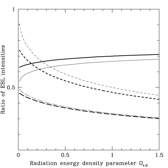Figure 3. Ratios Q / Q* (long-dashed lines), Qstat / Q* (short-dashed lines) and Q / Qstat (solid lines) as a function of radiation density r,0. Heavier lines are calculated for zf = 3 while lighter ones have zf = .

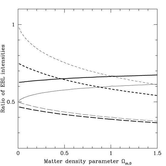Figure 4. Ratios Q / Q* (long-dashed lines), Qstat / Q* (short-dashed lines) and Q / Qstat (solid lines) as a function of matter density m,0. Heavier lines are calculated for zf = 3 while lighter ones have zf = .

Figs. 3 and 4 show that while the individual intensities Q / Q_* and Q_stat / Q_* do vary significantly with _r,0 and _m,0 in radiation- and matter-dominated models, their ratio Q / Q_stat remains nearly constant across the whole of the phase space, staying inside the range 0.5 Q / Q_stat 0.7 for both models.

Figure 5. Ratios Q / Q* (long-dashed lines), Qstat / Q* (short-dashed lines) and Q / Qstat (solid lines) as a function of vacuum energy density , 0. Heavier lines are calculated for zf = 3 while lighter ones have zf = for , 0 1 and zf = zmax for , 0 > 1. The dotted vertical line marks the maximum value of , 0 for which one can integrate to zf = 3.

Fig. 5 shows that a similar trend occurs in vacuum-dominated models. While absolute EBL intensities Q / Q_* and Q_stat / Q_* differ from those in the radiation- and matter-dominated models, their ratio (solid lines) is again close to flat. The exception occurs as _{, 0} 1 (de Sitter model), where i>Q / Q_stat dips well below 0.5 for large z_f. For _{, 0} > 1, there is no big bang (in models with _r,0 = _m,0 = 0), and one has instead a "big bounce" (i.e. a nonzero scale factor at the beginning of the expansionary phase). This implies a maximum possible redshift z_max given by

(48)

While such models are rarely considered, it is interesting to note that the same pattern persists here, albeit with one or two wrinkles. In light of (48), one can no longer integrate out to arbitarily high formation redshift z_f. If one wants to integrate to at least z_f, then one is limited to vacuum densities less than _{, 0} < (1 + z_f)² / [(1 + z_f)² - 1], or _{, 0} < 16/15 for the case z_f = 3 (heavy dotted line). More generally, for _{, 0} > 1 the limiting value of EBL intensity (shown with light lines) is reached as z_f z_max rather than z_f for both expanding and static models. Over the entire parameter space -0.5 _{, 0} 1.5 (except in the immediate vicinity of _{, 0} = 1), Fig. 5 shows that 0.4 Q / Q_stat 0.7 as before.

When more than one component of matter is present, analytic expressions can be found in only a few special cases, and the ratios Q / Q_* and Q_stat / Q_* must in general be computed numerically. We show the results in Fig. 6 for the situation which is of most physical interest: a universe containing both dust-like matter (_m,0, horizontal axis) and vacuum energy (_{, 0}, vertical axis), with _r,0 = 0.

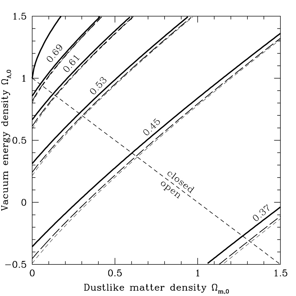Figure 6. The ratio Q / Q* in an expanding Universe, plotted as a function of matter density parameter m,0 and vacuum density parameter , 0 (with the radiation density parameter r,0 set to zero). Solid lines correspond to zf = 5, while long-dashed lines assume zf = 10 and short-dashed ones have zf = 50.

Fig. 6 shows that the bolometric intensity of the EBL is only modestly sensitive to the cosmological parameters _m,0 and _{, 0}. Moving from the lower right-hand corner of the phase space (Q / Q_* = 0.37) to the upper left-hand one (Q / Q_* = 0.69) changes the value of this quantity by less than a factor of two. Increasing the redshift of galaxy formation from z_f = 5 to 10 has little effect, and increasing it again to z_f = 50 even less. This means that, regardless of the redshift at which galaxies actually form, essentially all of the light reaching us from outside the Milky Way comes from galaxies at z < 5.

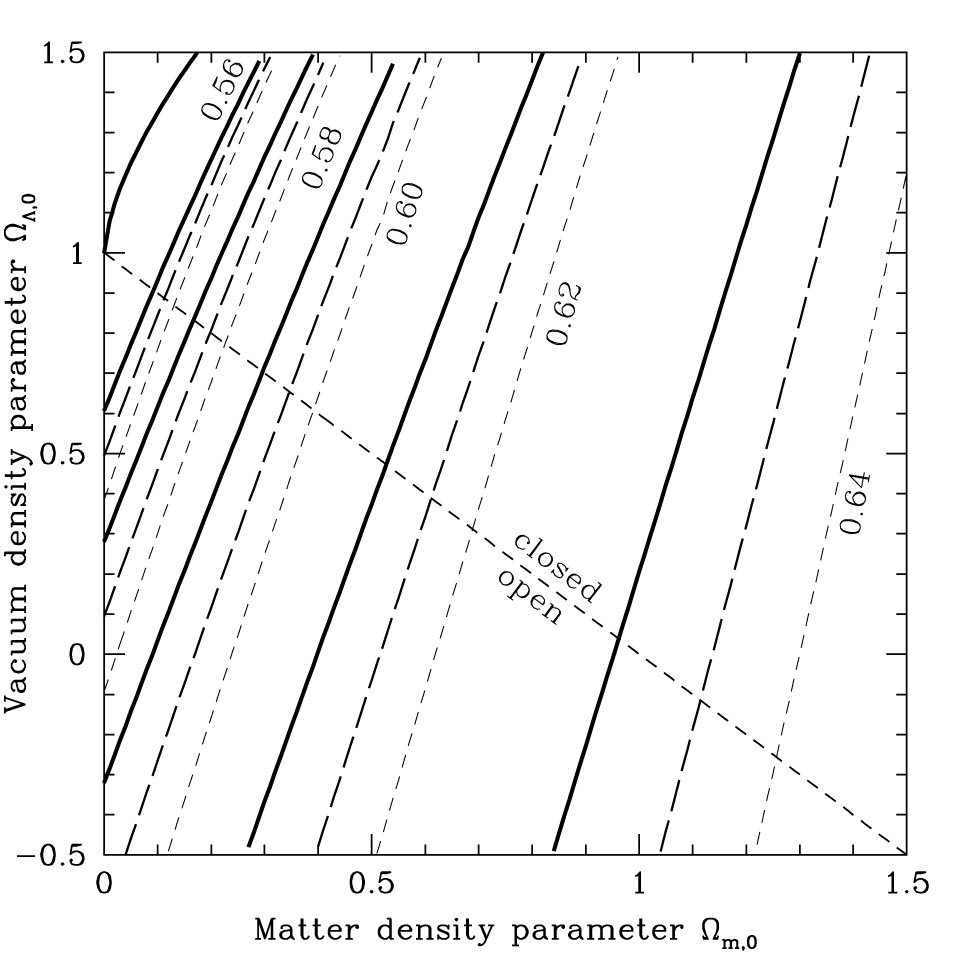Figure 7. The ratio Q / Qstat of EBL intensity in an expanding Universe to that in a static universe with the same values of the matter density parameter m,0 and vacuum density parameter , 0 (with the radiation density parameter r,0 set to zero). Solid lines correspond to zf = 4.5, while long-dashed lines assume zf = 5 and short-dashed ones have zf = 5.5.

While Fig. 6 confirms that the night sky is dark in any reasonable cosmological model, Fig. 7 shows why. It is a contour plot of Q / Q_stat, the value of which varies so little across the phase space that we have restricted the range of z_f-values to keep the diagram from getting too cluttered. The heavy (solid) lines are calculated for z_f = 4.5, the medium-weight (long-dashed) lines for z_f = 5, and the lightest (short-dashed) lines for z_f = 5.5. The spread in contour values is extremely narrow, from Q / Q_stat = 0.56 in the upper left-hand corner to 0.64 in the lower right-hand one -- a difference of less than 15%. Fig. 7 confirms our previous analytical results and leaves no doubt about the resolution of Olbers' paradox: the brightness of the night sky is determined to order of magnitude by the lifetime of the galaxies, and reduced by a factor of only 0.6 ± 0.1 due to the expansion of the Universe.

2.7. A look ahead

In this section, we inquire into the evolution of bolometric EBL intensity Q(t) with time, as specified mathematically by Eq. (12). Evaluation of this integral requires a knowledge of R(t), which is not well constrained by observation. Exact solutions are however available under the assumption that the Universe is spatially flat, as currently suggested by data on the power spectrum of fluctuations in the cosmic microwave background (Sec. 4). In this case k = 0 and (22) simplifies to

(49)

where we have taken = _r + _m in general and used (23) for . If one of these three components is dominant at a given time, then we can make use of (32) to obtain

(50)

These differential equations are solved to give

(51)

We emphasize that these expressions assume (i) spatial flatness, and (ii) a single-component cosmic fluid which must have the critical density.

Putting (51) into (12), we can solve for the bolometric intensity under the assumption that the luminosity of the galaxies is constant over their lifetimes, L(t) = L₀:

(52)

where we have used (21) and assumed that t_f << t₀ and t_f << t.

The intensity of the light reaching us from intergalactic space climbs as t ^3/2 in a radiation-filled Universe, t ^5/3 in a matter-dominated one, and exp(H₀ t) in one which contains only vacuum energy. This happens because the horizon of the Universe expands to encompass more and more galaxies, and hence more photons. Clearly it does so at a rate which more than compensates for the dilution and redshifting of existing photons due to expansion. Suppose for argument's sake that this state of affairs could continue indefinitely. How long would it take for the night sky to become as bright as, say, the interior of a typical living-room containing a single 100 W bulb and a summed surface area of 100 m² (Q_bulb = 1000 erg cm^-2 s^-1)?

The required increase of Q(t) over Q_* (= 2.5 × 10^-4 erg cm^-2 s^-1) is 4 million times. Eq. (52) then implies that

(53)

where we have taken H₀ t₀ 1 and t₀ 14 Gyr, as suggested by the observational data (Sec. 4). The last of the numbers in (53) is particularly intriguing. In a vacuum-dominated universe in which the luminosity of the galaxies could be kept constant indefinitely, the night sky would fill up with light over timescales of the same order as the theoretical hydrogen-burning lifetimes of the longest-lived stars. Of course, the luminosity of galaxies cannot stay constant over these timescales, because most of their light comes from much more massive stars which burn themselves out after tens of Gyr or less.

To check whether the situation just described is perhaps an artefact of the empty de Sitter universe, we require an expression for R(t) in models with both dust-like matter and vacuum energy. An analytic solution does exist for such models, if they are flat (i.e. _,0 = 1 - _m,0). It reads [1]:

(54)

This formula receives surprisingly little attention, given the importance of vacuum-dominated models in modern cosmology. Differentiation with respect to time gives the Hubble expansion rate:

(55)

This goes over to _{, 0}^1/2 as t , a result which (as noted in Sec. 2.3) holds quite generally for models with > 0. Alternatively, setting = (1 + z)^-1 in (54) gives the age of the Universe at a redshift z:

(56)

Setting z = 0 in this equation gives the present age of the Universe (t₀). Thus a model with (say) _m,0 = 0.3 and _{, 0} = 0.7 has an age of t₀ = 0.96H₀^-1 or, using (18), t₀ = 9.5h₀^-1 Gyr. Alternatively, in the limit _m,0 1, Eq. (56) gives back the standard result for the age of an EdS Universe, t₀ = 2 / (3H₀) = 6.5h₀^-1 Gyr.

Putting (54) into Eq. (12) with L(t) = L₀ = constant, and integrating over time, we obtain the plots of bolometric EBL intensity shown in Fig. 8. This diagram shows that the specter of a rapidly-brightening Universe does not occur only in the pure de Sitter model (short-dashed line). A model with an admixture of dust-like matter and vacuum energy such that _m,0 = 0.3 and _{, 0} = 0.7, for instance, takes only slightly longer (280 Gyr) to attain the "living-room" intensity of Q_bulb = 1000 erg cm^-2 s^-1.

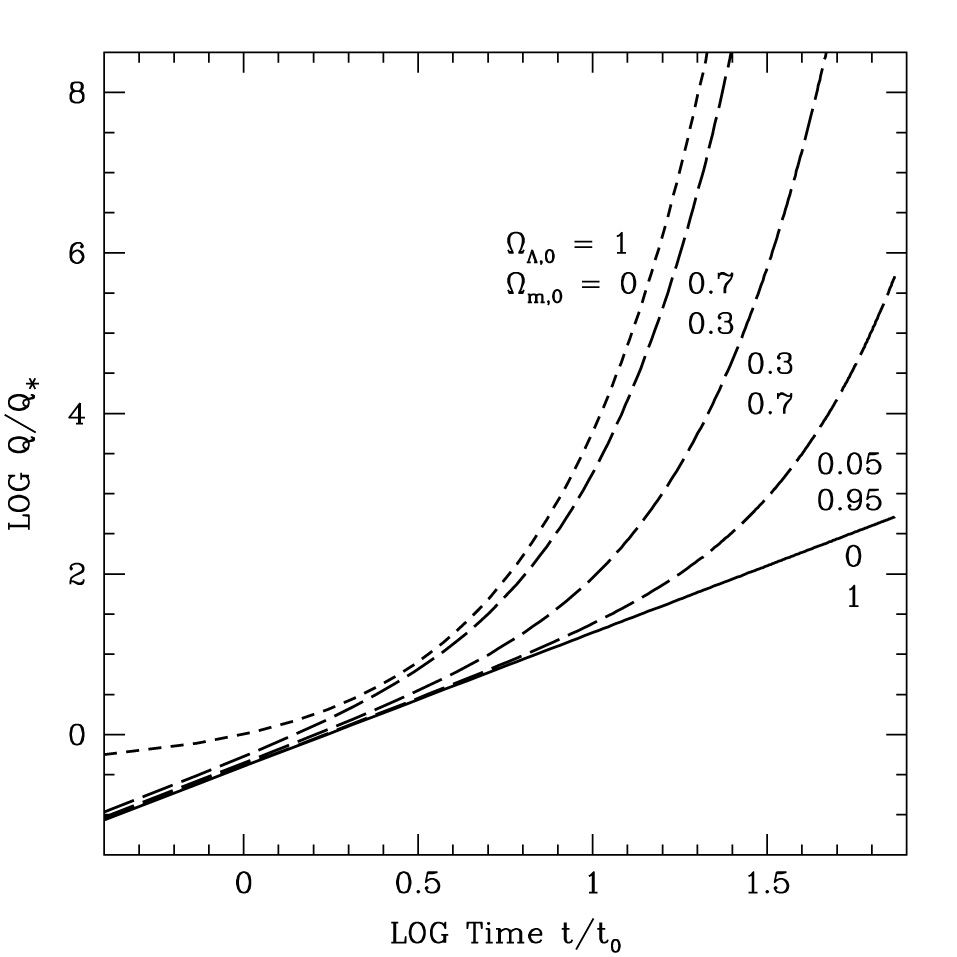Figure 8. Plots of Q(t) / Q* in flat models containing both dust-like matter (m,0) and vacuum energy (, 0). The solid line is the Einstein-de Sitter model, while the short-dashed line is pure de Sitter, and long-dashed lines represent intermediate models. The curves do not meet at t = t0 because Q(t0) differs from model to model, with Q(t0) = Q* only for the pure de Sitter case.