3. THE SPECTRUM OF COSMIC BACKGROUND RADIATION

3.1. Spectral intensity

The spectra of real galaxies depend strongly on wavelength and also evolve with time. How might these facts alter the conclusion obtained in Sec. 2; namely, that the brightness of the night sky is overwhelmingly determined by the age of the Universe, with expansion playing only a minor role?

The significance of this question is best appreciated in the microwave portion of the electromagnetic spectrum (at wavelengths from about 1 mm to 10 cm) where we know from decades of radio astronomy that the "night sky" is brighter than its optical counterpart (Fig. 1). The majority of this microwave background radiation is thought to come, not from the redshifted light of distant galaxies, but from the fading glow of the big bang itself -- the "ashes and smoke" of creation in Lemaître's words. Since its nature and suspected origin are different from those of the EBL, this part of the spectrum has its own name, the cosmic microwave background (CMB). Here expansion is of paramount importance, since the source radiation in this case was emitted at more or less a single instant in cosmological history (so that the "lifetime of the sources" is negligible). Another way to see this is to take expansion out of the picture, as we did in Sec. 2.4: the CMB intensity we would observe in this "equivalent static model" would be that of the primordial fireball and would roast us alive.

While Olbers' paradox involves the EBL, not the CMB, this example is still instructive because it prompts us to consider whether similar (though less pronounced) effects could have been operative in the EBL as well. If, for instance, galaxies emitted most of their light in a relatively brief burst of star formation at very early times, this would be a galactic approximation to the picture just described, and could conceivably boost the importance of expansion relative to lifetime, at least in some wavebands. To check on this, we need a way to calculate EBL intensity as a function of wavelength. This is motivated by other considerations as well. Olbers' paradox has historically been concerned primarily with the optical waveband (from approximately 4000Å to 8000Å), and this is still what most people mean when they refer to the "brightness of the night sky." And from a practical standpoint, we would like to compare our theoretical predictions with observational data, and these are necessarily taken using detectors which are optimized for finite portions of the electromagnetic spectrum.

We therefore adapt the bolometric formalism of Sec. 2. Instead of total luminosity L, consider the energy emitted by a source per unit time between wavelengths and + d. Let us write this in the form dL F(, t) d where F(, t) is the spectral energy distribution (SED), with dimensions of energy per unit time per unit wavelength. Luminosity is recovered by integrating the SED over all wavelengths:

(57)

We then return to (11), the bolometric intensity of the spherical shell of galaxies depicted in Fig. 2. Replacing L(t) with dL in this equation gives the intensity of light emitted between and + d:

(58)

This light reaches us at the redshifted wavelength ₀ = / (t). Redshift also stretches the wavelength interval by the same factor, d₀ = d / (t). So the intensity of light observed by us between ₀ and ₀ + d₀ is

(59)

The intensity of the shell per unit wavelength, as observed at wavelength ₀, is then given simply by

(60)

where the factor 4 converts from an all-sky intensity to one measured per steradian. (This is merely a convention, but has become standard.) Integrating over all the spherical shells corresponding to times t₀ and t₀ - t_f (as before) we obtain the spectral analog of our earlier bolometric result, Eq. (12):

(61)

This is the integrated light from many galaxies, which has been emitted at various wavelengths and redshifted by various amounts, but which is all in the waveband centered on ₀ when it arrives at us. We refer to this as the spectral intensity of the EBL at ₀. Eq. (61), or ones like it, have been considered from the theoretical side principally by McVittie and Wyatt [12], Whitrow and Yallop [13, 14] and Wesson [10, 15].

Eq. (61) can be converted from an integral over t to one over z by means of Eq. (14) as before. This gives

(62)

Eq. (62) is the spectral analog of (15). It may be checked using (57) that bolometric intensity is just the integral of spectral intensity over all observed wavelengths, Q = ₀ I(₀) d₀. Eqs. (61) and (62) provide us with the means to constrain any kind of radiation source by means of its contributions to the background light, once its number density n(z) and energy spectrum F(, z) are known. In subsequent sections we will apply them to various species of dark (or not so dark) energy and matter.

In this section, we return to the question of lifetime and the EBL. The static analog of Eq. (61) (i.e. the equivalent spectral EBL intensity in a universe without expansion, but with the properties of the galaxies unchanged) is obtained exactly as in the bolometric case by setting (t) = 1 (Sec. 2.4):

(63)

Just as before, we may convert this to an integral over z if we choose. The latter parameter no longer represents physical redshift (since this has been eliminated by hypothesis), but is now merely an algebraic way of expressing the age of the galaxies. This is convenient because it puts (63) into a form which may be directly compared with its counterpart (62) in the expanding Universe:

(64)

If the same values are adopted for H₀ and z_f, and the same functional forms are used for n(z), F(, z) and (z), then Eqs. (62) and (64) allow us to compare model universes which are alike in every way, except that one is expanding while the other stands still.

Some simplification of these expressions is obtained as before in situations where the comoving source number density can be taken as constant, n(z) = n₀. However, it is not possible to go farther and pull all the dimensional content out of these integrals, as was done in the bolometric case, until a specific form is postulated for the SED F(, z).

3.2. Comoving luminosity density

The simplest possible source spectrum is one in which all the energy is emitted at a single peak wavelength _p at each redshift z, thus

(65)

SEDs of this form are well-suited to sources of electromagnetic radiation such as elementary particle decays, which are characterized by specific decay energies and may occur in the dark-matter halos surrounding galaxies. The -function SED is not a realistic approximation for the spectra of galaxies themselves, but we will apply it here in this context to lay the foundation for later sections.

The function F_p(z) is obtained in terms of the total source luminosity L(z) by normalizing over all wavelengths

(66)

so that F_p(z) = L(z) / _p. In the case of galaxies, a logical choice for the characteristic wavelength _p would be the peak wavelength of a blackbody of "typical" stellar temperature. Taking the Sun as typical (T = T = 5770K), this would be _p = (2.90 mm K)/T = 5020Å from Wiens' law. Distant galaxies are seen chiefly during periods of intense starburst activity when many stars are much hotter than the Sun, suggesting a shift toward shorter wavelengths. On the other hand, most of the short-wavelength light produced in large starbursting galaxies (as much as 99% in the most massive cases) is absorbed within these galaxies by dust and re-radiated in the infrared and microwave regions ( 10, 000Å). It is also important to keep in mind that while distant starburst galaxies may be hotter and more luminous than local spirals and ellipticals, the latter contribute most to EBL intensity by virtue of their numbers at low redshift. The best that one can do with a single characteristic wavelength is to locate it somewhere within the B-band (3600 - 5500Å). For the purposes of this exercise we associate _p with the nominal center of this band, _p = 4400Å, corresponding to a blackbody temperature of 6590 K.

Substituting the SED (65) into the spectral intensity integral (62) leads to

(67)

where we have introduced a new shorthand for the comoving luminosity density of galaxies:

(68)

At redshift z = 0 this takes the value ₀, as given by (20). Numerous studies have shown that the product of n(z) and L(z) is approximately conserved with redshift, even when the two quantities themselves appear to be evolving markedly. So it would be reasonable to take (z) = ₀ = const. However, recent analyses have been able to benefit from observational work at deeper redshifts, and a consensus is emerging that (z) does rise slowly but steadily with z, peaking in the range 2 z 3, and falling away sharply thereafter [16]. This is consistent with a picture in which the first generation of massive galaxy formation occurred near z ~ 3, being followed at lower redshifts by galaxies whose evolution proceeded more passively.

Fig. 9 shows the value of ₀ from (20) at z = 0 [2] together with the extrapolation of (z) to five higher redshifts from an analysis of photometric galaxy redshifts in the Hubble Deep Field (HDF) [17]. We define a relative comoving luminosity density (z) by

(69)

and fit this to the data with a cubic [log(z) = z + z² + z³]. The best least-squares fit is plotted as a solid line in Fig. 9 along with upper and lower limits (dashed lines). We refer to these cases in what follows as the "moderate," "strong" and "weak" galaxy evolution scenarios respectively.

Figure 9. The comoving luminosity density of the Universe (z) (in h0 L Mpc-3), as observed at z = 0 (square) and extrapolated to higher redshifts based on analysis of the Hubble Deep Field (circles). The solid curve is a least-squares fit to the data; dashed lines represent upper and lower limits.

3.3. The delta-function spectrum

Inserting (69) into (67) puts the latter into the form

(70)

The dimensional content of this integral has been concentrated into a prefactor I, defined by

(71)

This constant shares two important properties of its bolometric counterpart Q_* (Sec. 2.2). First, it is independent of the uncertainty h₀ in Hubble's constant. Second, it is low by everyday standards. It is, for example, far below the intensity of the zodiacal light, which is caused by the scattering of sunlight by dust in the plane of the solar system. This is important, since the value of I sets the scale of the integral (70) itself. Indeed, existing observational bounds on I(₀) at ₀ 4400Å are of the same order as I. Toller, for example, set an upper limit of I(4400Å) < 4.5 × 10^-9erg s^-1 cm^-2 Å^-1 ster^-1 using data from the Pioneer 10 photopolarimeter [18].

Dividing I of (71) by the photon energy E₀ = hc / ₀ (where hc = 1.986 × 10^-8 erg Å) puts the EBL intensity integral (70) into new units, sometimes referred to as continuum units (CUs):

(72)

where 1 CU 1 photon s^-1 cm^-2 Å^-1 ster^-1. While both kinds of units (CUs and erg s^-1 cm^-2 Å^-1 ster^-1) are in common use for reporting spectral intensity at near-optical wavelengths, CUs appear most frequently. They are also preferable from a theoretical point of view, because they most faithfully reflect the energy content of a spectrum [19]. A third type of intensity unit, the S₁₀ (loosely, the equivalent of one tenth-magnitude star per square degree) is also occasionally encountered but will be avoided in this review as it is wavelength-dependent and involves other subtleties which differ between workers.

If we let the redshift of formation z_f then Eq. (70) reduces to

(73)

The comoving luminosity density (₀ / _p - 1) which appears here is fixed by the fit (69) to the HDF data in Fig. 9. The Hubble parameter is given by (33) as (₀ / _p -1) = [_m,0(₀ / _p)³ + _{, 0} - (_m,0 + _{, 0} -1)(₀ / _p)²]^1/2 for a universe containing dust-like matter and vacuum energy with density parameters _m,0 and _{, 0} respectively.

Turning off the luminosity density evolution (so that = 1 = const.), one obtains three trivial special cases:

(74)

These are taken at _{0 p}, where (_m,0, _{, 0}) = (1, 0),(0, 1) and (0, 0) respectively for the three models cited (Table 1). The first of these is the "7/2-law" which often appears in the particle-physics literature as an approximation to the spectrum of EBL contributions from decaying particles. But the second (de Sitter) probably provides a better approximation, given current thinking regarding the values of _m,0 and _{, 0}.

To evaluate the spectral EBL intensity (70) and other quantities in a general situation, it will be helpful to define a suite of cosmological test models which span the widest range possible in the parameter space defined by _m,0 and _{, 0}. We list four such models in Table 2 and summarize the main rationale for each here (see Sec. 4 for more detailed discussion). The Einstein-de Sitter (EdS) model has long been favoured on grounds of simplicity, and still sometimes referred to as the "standard cold dark matter" or SCDM model. It has come under increasing pressure, however, as evidence mounts for levels of _m,0 0.5, and most recently from observations of Type Ia supernovae (SNIa) which indicate that _{, 0} > _m,0. The Open Cold Dark Matter (OCDM) model is more consistent with data on _m,0 and holds appeal for those who have been reluctant to accept the possibility of a nonzero vacuum energy. It faces the considerable challenge, however, of explaining data on the spectrum of CMB fluctuations, which imply that _m,0 + _{, 0} 1. The +Cold Dark Matter (CDM) model has rapidly become the new standard in cosmology because it agrees best with both the SNIa and CMB observations. However, this model suffers from a "coincidence problem," in that _m(t) and (t) evolve so differently with time that the probability of finding ourselves at a moment in cosmic history when they are even of the same order of magnitude appears unrealistically small. This is addressed to some extent in the last model, where we push _m,0 and _{, 0} to their lowest and highest limits, respectively. In the case of _m,0 these limits are set by big-bang nucleosynthesis, which requires a density of at least _m,0 0.03 in baryons (hence the +Baryonic Dark Matter or BDM model). Upper limits on _{, 0} come from various arguments, such as the observed frequency of gravitational lenses and the requirement that the Universe began in a big-bang singularity. Within the context of isotropic and homogeneous cosmology, these four models cover the full range of what would be considered plausible by most workers.

Table 2. Cosmological test models

	EdS/SCDM	OCDM	CDM	BDM
m,0	1	0.3	0.3	0.03
, 0	0	0	0.7	1

Fig. 10 shows the solution of the full integral (70) for all four test models, superimposed on a plot of available experimental data at near-optical wavelengths (i.e. a close-up of Fig. 1). The short-wavelength cutoff in these plots is an artefact of the -function SED, but the behaviour of I(₀) at wavelengths above _p = 4400 Å is quite revealing, even in a model as simple as this one. In the EdS case (a), the rapid fall-off in intensity with ₀ indicates that nearby (low-redshift) galaxies dominate. There is a secondary hump at ₀ 10, 000 Å, which is an "echo" of the peak in galaxy formation, redshifted into the near infrared. This hump becomes progressively larger relative to the optical peak at 4400 Å as the ratio of _{, 0} to _m,0 grows. Eventually one has the situation in the de Sitter-like model (d), where the galaxy-formation peak entirely dominates the observed EBL signal, despite the fact that it comes from distant galaxies at z 3. This is because a large _{, 0}-term (especially one which is large relative to _m,0) inflates comoving volume at high redshifts. Since the comoving number density of galaxies is fixed by the fit to observational data on (z) (Fig. 9), the number of galaxies at these redshifts must go up, pushing up the infrared part of the spectrum. Although the -function spectrum is an unrealistic one, we will see that this trend persists in more sophisticated models, providing a clear link between observations of the EBL and the cosmological parameters _m,0 and _,0.

Figure 10. The spectral EBL intensity of galaxies whose radiation is modelled by -functions at a rest frame wavelength of 4400Å, calculated for four different cosmological models: (a) EdS, (b) OCDM, (c) CDM and (d) BDM (Table 2). Also shown are observational upper limits (solid symbols and heavy lines) and reported detections (empty symbols) over the waveband 2000-40,000Å.

Fig. 10 is plotted over a broad range of wavelengths from the near ultraviolet (NUV; 2000-4000Å) to the near infrared (NIR; 8000-40,000Å). The upper limits in this plot (solid symbols and heavy lines) come from analyses of OAO-2 satellite data (LW76 [20]), ground-based telescopes (SS78 [21], D79 [22], BK86 [23]), Pioneer 10 (T83 [18]), sounding rockets (J84 [24], T88 [25]), the shuttle-borne Hopkins UVX (M90 [26]) and -- in the near infrared -- the DIRBE instrument aboard the COBE satellite (H98 [27]). The past few years have also seen the first widely-accepted detections of the EBL (Fig. 10, open symbols). In the NIR these have come from continued analysis of DIRBE data in the K-band (22,000Å) and L-band (35,000Å; WR00 [28]), as well as the J-band (12,500Å; C01 [29]). Reported detections in the optical using a combination of Hubble Space Telescope (HST) and Las Campanas telescope observations (B02 [30]) are preliminary [31] but potentially very important.

Fig. 10 shows that EBL intensities based on the simple -function spectrum are in rough agreement with these data. Predicted intensities come in at or just below the optical limits in the low-_{, 0} cases (a) and (b), and remain consistent with the infrared limits even in the high-_{, 0} cases (c) and (d). Vacuum-dominated models with even higher ratios of _{, 0} to _m,0 would, however, run afoul of DIRBE limits in the J-band.

3.4. The Gaussian spectrum

The Gaussian distribution provides a useful generalization of the -function for modelling sources whose spectra, while essentially monochromatic, are broadened by some physical process. For example, photons emitted by the decay of elementary particles inside dark-matter halos would have their energies Doppler-broadened by circular velocities v_c 220 km s^-1, giving rise to a spread of order () = (2v_c / c) 0.0015 in the SED. In the context of galaxies, this extra degree of freedom provides a simple way to model the width of the bright part of the spectrum. If we take this to cover the B-band (3600-5500Å) then ~ 1000Å. The Gaussian SED reads

(75)

where _p is the wavelength at which the galaxy emits most of its light. We take _p = 4400Å as before, and note that integration over ₀ confirms that L(z) = ₀ F(, z) d as required. Once again we can make the simplifying assumption that L(z) = L₀ = const., or we can use the empirical fit (z) n(z) L(z) / ₀ to the HDF data in Fig. 9. Taking the latter course and substituting (75) into (62), we obtain

(76)

The dimensional content of this integral has been pulled into a prefactor I_g = I_g(₀), defined by

(77)

Here we have divided (76) by the photon energy E₀ = hc / ₀ to put the result into CUs, as before.

Results are shown in Fig. 11, where we have taken _p = 4400Å, = 1000Å and z_f = 6. Aside from the fact that the short-wavelength cutoff has disappeared, the situation is qualitatively similar to that obtained using a -function approximation. (This similarity becomes formally exact as approaches zero.) One sees, as before, that the expected EBL signal is brightest at optical wavelengths in an EdS Universe (a), but that the infrared hump due to the redshifted peak of galaxy formation begins to dominate for higher-_{, 0} models (b) and (c), becoming overwhelming in the de Sitter-like model (d). Overall, the best agreement between calculated and observed EBL levels occurs in the CDM model (c). The matter-dominated EdS (a) and OCDM (b) models contain too little light (requiring one to postulate an additional source of optical or near-optical background radiation besides that from galaxies), while the BDM model (d) comes uncomfortably close to containing too much light. This is an interesting situation, and one which motivates us to reconsider the problem with more realistic models for the galaxy SED.

Figure 11. The spectral EBL intensity of galaxies whose spectra has been represented by Gaussian distributions with rest frame peak wavelength 4400Å and standard deviation 1000Å, calculated for the (a) EdS, (b) OCDM, (c) CDM and (d) BDM cosmologies and compared with observational upper limits (solid symbols and heavy lines) and reported detections (empty symbols).

3.5. The Planckian spectrum

The simplest nontrivial approach to a galaxy spectrum is to model it as a blackbody, and this was done by previous workers such as McVittie and Wyatt [12], Whitrow and Yallop [13, 14] and Wesson [15]. Let us suppose that the galaxy SED is a product of the Planck function and some wavelength-independent parameter C(z):

(78)

Here _SB 2⁵ k⁴ / 15c² h³ = 5.67 × 10^-5 erg cm^-2 s^-1 K^-1 is the Stefan-Boltzmann constant. The function F is normally regarded as an increasing function of redshift (at least out to the redshift of galaxy formation). This can in principle be accommodated by allowing C(z) or T(z) to increase with z in (78). The former choice would correspond to a situation in which galaxy luminosity decreases with time while its spectrum remains unchanged, as might happen if stars were simply to die. The second choice corresponds to a situation in which galaxy luminosity decreases with time as its spectrum becomes redder, as may happen when its stellar population ages. The latter scenario is more realistic, and will be adopted here. The luminosity L(z) is found by integrating F(, z) over all wavelengths:

(79)

so that the unknown function C(z) must satisfy C(z) = L(z) / [T(z)] ⁴. If we require that Stefan's law (L T⁴) hold at each z, then

(80)

where T₀ is the present "galaxy temperature" (i.e. the blackbody temperature corresponding to a peak wavelength in the B-band). Thus the evolution of galaxy luminosity in this model is just that which is required by Stefan's law for blackbodies whose temperatures evolve as T(z). This is reasonable, since galaxies are made up of stellar populations which cool and redden with time as hot massive stars die out.

Let us supplement this with the assumption of constant comoving number density, n(z) = n₀ = const. This is sometimes referred to as the pure luminosity evolution or PLE scenario, and while there is some controversy on this point, PLE has been found by many workers to be roughly consistent with observed numbers of galaxies at faint magnitudes, especially if there is a significant vacuum energy density _{, 0} > 0. Proceeding on this assumption, the comoving galaxy luminosity density can be written

(81)

This expression can then be inverted for blackbody temperature T(z) as a function of redshift, since the form of (z) is fixed by Fig. 9:

(82)

We can check this by choosing T₀ = 6600K (i.e. a present peak wavelength of 4400Å) and reading off values of (z) = (z) / ₀ at the peaks of the curves marked "weak," "moderate" and "strong" evolution in Fig. 9. Putting these numbers into (82) yields blackbody temperatures (and corresponding peak wavelengths) of 10,000K (2900Å), 11,900K (2440Å) and 13,100K (2210Å) respectively at the galaxy-formation peak. These numbers are consistent with the idea that galaxies would have been dominated by hot UV-emitting stars at this early time.

Inserting the expressions (80) for C(z) and (82) for T(z) into the SED (78), and substituting the latter into the EBL integral (62), we obtain

(83)

The dimensional prefactor I_b = I_b(T₀, ₀) reads in this case

(84)

This integral is evaluated and plotted in Fig. 12, where we have set z_f = 6 following recent observational hints of an epoch of "first light" at this redshift [32]. Overall EBL intensity is insensitive to this choice, provided that z_f 3. Between z_f = 3 and z_f = 6, I(₀) rises by less than 1% below ₀ = 10,000Å and less than ~ 5% at ₀ = 20,000Å (where most of the signal originates at high redshifts). There is no further increase beyond z_f > 6 at the three-figure level of precision.

Figure 12. The spectral EBL intensity of galaxies, modelled as blackbodies whose characteristic temperatures are such that their luminosities L T4 combine to produce the observed comoving luminosity density (z) of the Universe. Results are shown for the (a) EdS, (b) OCDM, (c) CDM and (d) BDM cosmologies. Also shown are observational upper limits (solid symbols and heavy lines) and reported detections (open symbols).

Fig. 12 shows some qualitative differences from our earlier results obtained using -function and Gaussian SEDs. Most noticeably, the prominent "double-hump" structure is no longer apparent. The key evolutionary parameter is now blackbody temperature T(z) and this goes as [(z)],^1/4 so that individual features in the comoving luminosity density profile are suppressed. (A similar effect can be achieved with the Gaussian SED by choosing larger values of .) As before, however, the long-wavelength part of the spectrum climbs steadily up the right-hand side of the figure as one moves from the _{, 0} = 0 models (a) and (b) to the _{, 0}-dominated models (c) and (d), whose light comes increasingly from more distant, redshifted galaxies.

Absolute EBL intensities in each of these four models are consistent with what we have seen already. This is not surprising, because changing the shape of the SED merely shifts light from one part of the spectrum to another. It cannot alter the total amount of light in the EBL, which is set by the comoving luminosity density (z) of sources once the background cosmology (and hence the source lifetime) has been chosen. As before, the best match between calculated EBL intensities and the observational detections is found for the _{, 0}-dominated models (c) and (d). The fact that the EBL is now spread across a broader spectrum has pulled down its peak intensity slightly, so that the BDM model (d) no longer threatens to violate observational limits and in fact fits them rather nicely. The zero-_{, 0} models (a) and (b) again appear to require some additional source of background radiation (beyond that produced by galaxies) if they are to contain enough light to make up the levels of EBL intensity that have been reported.

3.6. Normal and starburst galaxies

The previous sections have shown that simple models of galaxy spectra, combined with data on the evolution of comoving luminosity density in the Universe, can produce levels of spectral EBL intensity in rough agreement with observational limits and reported detections, and even discriminate to a degree between different cosmological models. However, the results obtained up to this point are somewhat unsatisfactory in that they are sensitive to theoretical input parameters, such as _p and T₀, which are hard to connect with the properties of the actual galaxy population.

A more comprehensive approach would use observational data in conjunction with theoretical models of galaxy evolution to build up an ensemble of evolving galaxy SEDs F(, z) and comoving number densities n(z) which would depend not only on redshift but on galaxy type as well. Increasingly sophisticated work has been carried out along these lines over the years by Partridge and Peebles [33], Tinsley [34], Bruzual [35], Code and Welch [36], Yoshii and Takahara [37] and others. The last-named authors, for instance, divided galaxies into five morphological types (E/SO, Sab, Sbc, Scd and Sdm), with a different evolving SED for each type, and found that their collective EBL intensity at NIR wavelengths was about an order of magnitude below the levels suggested by observation.

Models of this kind, however, are complicated while at the same time containing uncertainties. This makes their use somewhat incompatible with our purpose here, which is primarily to obtain a first-order estimate of EBL intensity so that the importance of expansion can be properly ascertained. Also, observations have begun to show that the above morphological classifications are of limited value at redshifts z 1, where spirals and ellipticals are still in the process of forming [38]. As we have already seen, this is precisely where much of the EBL may originate, especially if luminosity density evolution is strong, or if there is a significant _{, 0}-term.

What is needed, then, is a simple model which does not distinguish too finely between the spectra of galaxy types as they have traditionally been classified, but which can capture the essence of broad trends in luminosity density evolution over the full range of redshifts 0 z z_f. For this purpose we will group together the traditional classes (spiral, elliptical, etc.) under the single heading of quiescent or normal galaxies. At higher redshifts (z 1), we will allow a second class of objects to play a role: the active or starburst galaxies. Whereas normal galaxies tend to be comprised of older, redder stellar populations, starburst galaxies are dominated by newly-forming stars whose energy output peaks in the ultraviolet (although much of this is absorbed by dust grains and subsequently reradiated in the infrared). One signature of the starburst type is thus a decrease in F() as a function of over NUV and optical wavelengths, while normal types show an increase [39]. Starburst galaxies also tend to be brighter, reaching bolometric luminosities as high as 10¹² - 10¹³ L, versus 10¹⁰ - 10¹¹ L for normal types.

There are two ways to obtain SEDs for these objects: by reconstruction from observational data, or as output from theoretical models of galaxy evolution. The former approach has had some success, but becomes increasingly difficult at short wavelengths, so that results have typically been restricted to 1000Å [39]. This represents a serious limitation if we want to integrate out to redshifts z_f ~ 6 (say), since it means that our results are only strictly reliable down to ₀ = (1 + z_f) ~ 7000Å. In order to integrate out to z_f ~ 6 and still go down as far as the NUV (₀ ~ 2000Å), we require SEDs which are good to ~ 300Å in the galaxy rest-frame. For this purpose we will make use of theoretical galaxy-evolution models, which have advanced to the point where they cover the entire spectrum from the far ultraviolet to radio wavelengths. This broad range of wavelengths involves diverse physical processes such as star formation, chemical evolution, and (of special importance here) dust absorption of ultraviolet light and re-emission in the infrared. Typical normal and starburst galaxy SEDs based on such models are now available down to ~ 100Å [40]. These functions, displayed in Fig. 13, will constitute our normal and starburst galaxy SEDs, F_n() and F_s().

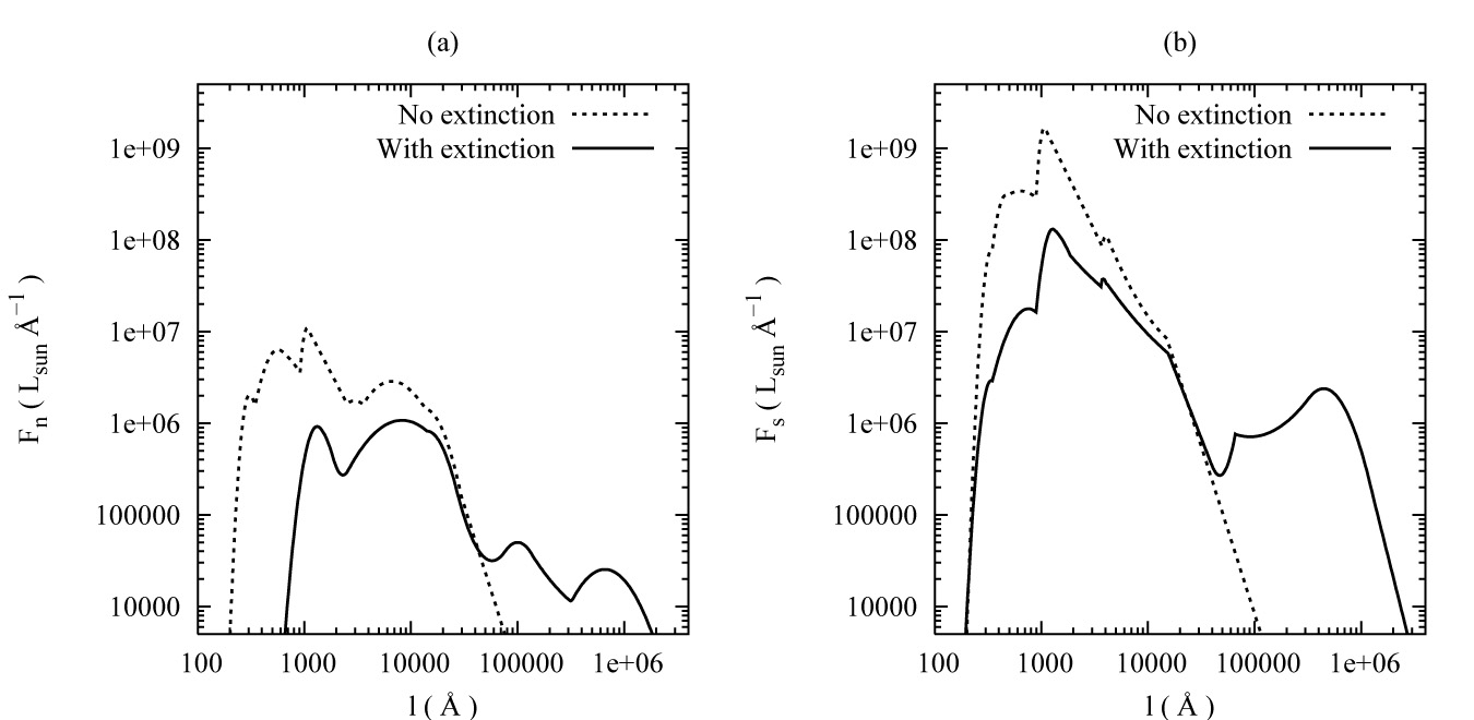Figure 13. Typical galaxy SEDs for (a) normal and (b) starburst type galaxies with and without extinction by dust. These figures are adapted from Figs. 9 and 10 of Devriendt [40]. For definiteness we have normalized (over 100 - 3 × 10 4Å) such that Ln = 1 × 1010 h0-2 L and Ls = 2 × 1011 h0-2 L with h0 = 0.75. (These values are consistent with what we will later call "model 0" for a comoving galaxy number density of n0 = 0.010 h03 Mpc-3.)

Fig. 13 shows the expected increase in F_n() with at NUV wavelengths (~ 2000Å) for normal galaxies, as well as the corresponding decrease for starbursts. What is most striking about both templates, however, is their overall multi-peaked structure. These objects are far from pure blackbodies, and the primary reason for this is dust. This effectively removes light from the shortest-wavelength peaks (which are due mostly to star formation), and transfers it to the longer-wavelength ones. The dashed lines in Fig. 13 show what the SEDs would look like if this dust reprocessing were ignored. The main difference between normal and starburst types lies in the relative importance of this process. Normal galaxies emit as little as 30% of their bolometric intensity in the infrared, while the equivalent fraction for the largest starburst galaxies can reach 99%. Such variations can be incorporated by modifying input parameters such as star formation timescale and gas density, leading to spectra which are broadly similar in shape to those in Fig. 13 but differ in normalization and "tilt" toward longer wavelengths. The results have been successfully matched to a wide range of real galaxy spectra [40].

3.7. Comparison with observation

We proceed to calculate the spectral EBL intensity using F_n() and F_s(), with the characteristic luminosities of these two types found as usual by normalization, F_n() d = L_n and F_s() d = L_s. Let us assume that the comoving luminosity density of the Universe at any redshift z is a combination of normal and starburst components

(85)

where comoving number densities are

(86)

In other words, we will account for evolution in (z) solely in terms of a changing starburst fraction f (z), and a single comoving number density n(z) as before. L_n and L_s are awkward to work with for dimensional reasons, and we will find it more convenient to specify the SED instead by two dimensionless parameters, the local starburst fraction f₀ and luminosity ratio ₀:

(87)

Observations indicate that f₀ 0.05 in the local population [39], and the SEDs shown in Fig. 13 have been fitted to a range of normal and starburst galaxies with 40 ₀ 890 [40]. We will allow these two parameters to vary in the ranges 0.01 f₀ 0.1 and 10 ₀ 1000. This, in combination with our "strong" and "weak" limits on luminosity-density evolution, gives us the flexibility to obtain upper and lower bounds on EBL intensity.

The functions n(z) and f (z) can now be fixed by equating (z) as defined by (85) to the comoving luminosity-density curves inferred from HDF data (Fig. 9), and requiring that f 1 at peak luminosity (i.e. assuming that the galaxy population is entirely starburst-dominated at the redshift z_p of peak luminosity). These conditions are not difficult to set up. One finds that modest number-density evolution is required in general, if f (z) is not to over- or under-shoot unity at z_p. We follow [42] and parametrize this with the function n(z) = n₀(1 + z) for z z_p. Here is often termed the merger parameter since a value of > 0 would imply that the comoving number density of galaxies decreases with time.

Pulling these requirements together, one obtains a model with

			(88)

Here (z) [1 / ₀ + (1 - 1 / ₀) f₀] (z) and = ln[(z_p)] / ln(1 + z_p). The evolution of f (z), n_n(z) and n_s(z) is plotted in Fig. 14 for five models: a best-fit Model 0, corresponding to the moderate evolution curve in Fig. 9 with f₀ = 0.05 and ₀ = 20, and four other models chosen to produce the widest possible spread in EBL intensities across the optical band. Models 1 and 2 are the most starburst-dominated, with initial starburst fraction and luminosity ratio at their upper limits (f₀ = 0.1 and ₀ = 1000). Models 3 and 4 are the least starburst-dominated, with the same quantities at their lower limits (f₀ = 0.01 and ₀ = 10). Luminosity density evolution is set to "weak" in the odd-numbered Models 1 and 3, and "strong" in the even-numbered Models 2 and 4. (In principle one could identify four other "extreme" combinations, such as maximum f₀ with minimum ₀, but these will be intermediate to Models 1-4.) We find merger parameters between +0.4, 0.5 in the strong-evolution Models 2 and 4, and -0.5, - 0.4 in the weak-evolution Models 1 and 3, while = 0 for Model 0. These are well within the normal range [43].

Figure 14. Evolution of (a) starburst fraction f (z) and (b) comoving normal and starburst galaxy number densities nn(z) and ns(z), where total comoving luminosity density (z) = nn(z)Ln + ns(z)Ls is matched to the "moderate," "weak" and "strong" evolution curves in Fig. 9. Each model has different values of the two adjustable parameters f0 f (0) and 0 Ls / Ln.

The information contained in Fig. 14 can be summarized in words as follows: starburst galaxies formed near z_f ~ 4 and increased in comoving number density until z_p ~ 2.5 (the redshift of peak comoving luminosity density in Fig. 9). They then gave way to a steadily growing population of fainter normal galaxies which began to dominate between 1 z 2 (depending on the model) and now make up 90-99% of the total galaxy population at z = 0. This scenario is in good agreement with others that have been constructed to explain the observed faint blue excess in galaxy number counts [41].

We are now in a position to compute the total spectral EBL intensity by substituting the SEDs (F_n, F_s) and comoving number densities (86) into Eq. (62). Results can be written in the form I(₀) = Iⁿ(₀) + I^s(₀) where:

			(89)

Here Iⁿ and I^s represent contributions from normal and starburst galaxies respectively and (z) n(z) / n₀ is the relative comoving number density. The dimensional content of both integrals has been pulled into a prefactor

(90)

This is independent of h₀, as before, because the factor of h₀ in ₀ cancels out the one in H₀. The quantity ₀ appears here when we normalize the galaxy SEDs F_n() and F_s() to the observed comoving luminosity density of the Universe. To see this, note that Eq. (85) reads ₀ = n₀ L_n[1 + (₀ - 1) f₀] at z = 0. Since ₀ n₀ L₀, it follows that L_n = L₀ / [1 + (₀ - 1) f₀] and L_s = L_{0 0} / [1 + (₀ - 1) f₀]. Thus a factor of L₀ can be divided out of the functions F_n and F_s and put directly into Eq. (89) as required.

The spectral intensity (89) is plotted in Fig. 15, where we have set z_f = 6 as usual. (Results are insensitive to this choice, increasing by less than 5% as one moves from z_f = 3 to z_f = 6, with no further increase for z_f 6 at three-figure precision.) These plots show that the most starburst-dominated models (1 and 2) produce the bluest EBL spectra, as might be expected. For these two models, EBL contributions from normal galaxies remain well below those from starbursts at all wavelengths, so that the bump in the observed spectrum at ₀ ~ 4000Å is essentially an echo of the peak at ~ 1100Å in the starburst SED (Fig. 13), redshifted by a factor (1 + z_p) from the epoch z_p 2.5 of maximum comoving luminosity density. By contrast, in the least starburst-dominated models (3 and 4), EBL contributions from normal galaxies catch up to and exceed those from starbursts at ₀ 10, 000Å, giving rise to the bump seen at ₀ ~ 20, 000Å in these models. Absolute EBL intensities are highest in the strong-evolution models (2 and 4) and lowest in the weak-evolution models (1 and 3). We emphasize that the total amount of light in the EBL is determined by the choice of luminosity density profile (for a given cosmological model). The choice of SED merely shifts this light from one part of the spectrum to another. Within the context of the simple two-component model described above, and the constraints imposed on luminosity density by the HDF data (Sec. 3.2), the curves in Fig. 15 represent upper and lower limits on the spectral intensity of the EBL at near-optical wavelengths.

Figure 15. The spectral EBL intensity of a combined population of normal and starburst galaxies, with SEDs as shown in Fig. 13. The evolving number densities are such as to reproduce the total comoving luminosity density seen in the HDF (Fig. 9). Results are shown for the (a) EdS, (b) OCDM, (c) CDM and (d) BDM cosmologies. Also shown are observational upper limits (solid symbols and heavy lines) and reported detections (open symbols).

These curves are spread over a broader range of wavelengths than those obtained earlier using single-component Gaussian and blackbody spectra. This leads to a drop in overall intensity, as we can appreciate by noting that there now appears to be a significant gap between theory and observation in all but the most vacuum-dominated cosmology, BDM (d). This is so even for the models with the strongest luminosity density evolution (models 2 and 4). In the case of the EdS cosmology (a), this gap is nearly an order of magnitude, as reported by Yoshii and Takahara [37]. Similar conclusions have been reached more recently from an analysis of Subaru Deep Field data by Totani [44], who suggest that the shortfall could be made up by a very diffuse, previously undetected component of background radiation not associated with galaxies. Other workers have argued that existing galaxy populations are enough to explain the data if different assumptions are made about their SEDs [45], or if allowance is made for faint low surface brightness galaxies below the detection limit of existing surveys [46].

3.8. Spectral resolution of Olbers' paradox

Having obtained quantitative estimates of the spectral EBL intensity which are in reasonable agreement with observation, we return to the question posed in Sec. 2.4: why precisely is the sky dark at night? By "dark" we now mean specifically dark at near-optical wavelengths. We can provide a quantitative answer to this question by using a spectral version of our previous bolometric argument. That is, we compute the EBL intensity I_,stat in model universes which are equivalent to expanding ones in every way except expansion, and then take the ratio I / I_,stat. If this is of order unity, then expansion plays a minor role and the darkness of the optical sky (like the bolometric one) must be attributed mainly to the fact that the Universe is too young to have filled up with light. If I / I_,stat << 1, on the other hand, then we would have a situation qualitatively different from the bolometric one, and expansion would play a crucial role in the resolution to Olbers' paradox.

The spectral EBL intensity for the equivalent static model is obtained by putting the functions (z), f (z), F_n(), F_s() and (z) into (64) rather than (62). This results in I_,stat(₀) = Iⁿ_,stat(₀) + I^s_,stat(₀) where normal and starburst contributions are given by

			(91)

Despite a superficial resemblance to their counterparts (89) in the expanding Universe, these are vastly different expressions. Most importantly, the SEDs F_n(₀) and F_s(₀) no longer depend on z and have been pulled out of the integrals. The quantity I_,stat(₀) is effectively a weighted mean of the SEDs F_n(₀) and F_s(₀). The weighting factors (i.e. the integrals over z) are related to the age of the galaxies, ₀^z_f dz / (1 + z) (z), but modified by factors of n_n(z) and n_s(z) under the integral. This latter modification is important because it prevents the integrals from increasing without limit as z_f becomes arbitrarily large, a problem that would otherwise introduce considerable uncertainty into any attempt to put bounds on the ratio I_,stat / I [15]. A numerical check confirms that I_,stat is nearly as insensitive to the value of z_f as I, increasing by up to 8% as one moves from z_f = 3 to z_f = 6, but with no further increase for z_f 6 at the three-figure level.

Figure 16. The ratio I / I,stat of spectral EBL intensity in expanding models to that in equivalent static models, for the (a) EdS, (b) OCDM, (c) CDM and (d) BDM models. The fact that this ratio lies between 0.3 and 0.6 in the B-band (4000-5000Å) tells us that expansion reduces the intensity of the night sky at optical wavelengths by a factor of between two and three.

The ratio of I / I_,stat is plotted over the waveband 2000-25,000Å in Fig. 16, where we have set z_f = 6. (Results are insensitive to this choice, as we have mentioned above, and it may be noted that they are also independent of uncertainty in constants such as ₀ since these are common to both I and I_,stat.) Several features in this figure deserve notice. First, the average value of I / I_,stat across the spectrum is about 0.6, consistent with bolometric expectations (Sec. 2). Second, the diagonal, bottom-left to top-right orientation arises largely because I(₀) drops off at short wavelengths, while I_,stat(₀) does so at long ones. The reason why I(₀) drops off at short wavelengths is that ultraviolet light reaches us only from the nearest galaxies; anything from more distant ones is redshifted into the optical. The reason why I_,stat(₀) drops off at long wavelengths is because it is a weighted mixture of the galaxy SEDs, and drops off at exactly the same place that they do: ₀ ~ 3 × 10⁴Å. In fact, the weighting is heavily tilted toward the dominant starburst component, so that the two sharp bends apparent in Fig. 16 are essentially (inverted) reflections of features in F_s(₀); namely, the small bump at ₀ ~ 4000Å and the shoulder at ₀ ~ 11, 000Å (Fig. 13).

Finally, the numbers: Fig. 16 shows that the ratio of I / I_,stat is remarkably consistent across the B-band (4000-5000Å) in all four cosmological models, varying from a high of 0.46 ± 0.10 in the EdS model to a low of 0.39 ± 0.08 in the BDM model. These numbers should be compared with the bolometric result of Q / Q_stat 0.6 ± 0.1 from Sec. 2. They tell us that expansion does play a greater role in determining B-band EBL intensity than it does across the spectrum as a whole -- but not by much. If its effects were removed, the night sky at optical wavelengths would be anywhere from two times brighter (in the EdS model) to three times brighter (in the BDM model). These results depend modestly on the makeup of the evolving galaxy population, and Fig. 16 shows that I / I_,stat in every case is highest for the weak-evolution model 1, and lowest for the strong-evolution model 4. This is as we would expect, based on our discussion at the beginning of this section: models with the strongest evolution effectively "concentrate" their light production over the shortest possible interval in time, so that the importance of the lifetime factor drops relative to that of expansion. Our numerical results, however, prove that this effect cannot qualitatively alter the resolution of Olbers' paradox. Whether expansion reduces the background intensity by a factor of two or three, its order of magnitude is still set by the lifetime of the Universe.

There is one factor which we have not considered in this section, and that is the extinction of photons by intergalactic dust and neutral hydrogen, both of which are strongly absorbing at ultraviolet wavelengths. The effect of this would primarily be to remove ultraviolet light from high-redshift galaxies and transfer it into the infrared -- light that would otherwise be redshifted into the optical and contribute to the EBL. The latter's intensity I(₀) would therefore drop, and one could expect reductions over the B-band in particular. The importance of this effect is difficult to assess because we have limited data on the character and distribution of dust beyond our own galaxy. We will find indications in Sec. 7, however, that the reduction could be significant at the shortest wavelengths considered here (₀ 2000Å) for the most extreme dust models. This would further widen the gap between observed and predicted EBL intensities noted at the end of Sec. 3.6.

Absorption plays far less of a role in the equivalent static models, where there is no redshift. (Ultraviolet light is still absorbed, but the effect does not carry over into the optical). Therefore, the ratio I / I_,stat would be expected to drop in nearly direct proportion to the drop in I. In this sense Olbers had part of the solution after all -- not (as he thought) because intervening matter "blocks" the light from distant sources, but because it transfers it out of the optical. The importance of this effect, which would be somewhere below that of expansion, is a separate issue from the one we have concerned ourselves with in this section. We have shown that expansion reduces EBL intensity by a factor of between two and three, depending on background cosmology and the evolutionary properties of the galaxy population. Thus the optical sky, like the bolometric one, is dark at night primarily because it has not had enough time to fill up with light from distant galaxies.