3. COSMIC STAR FORMATION HISTORIES

3.1. When Did Galaxies Form? Searches for Primeval Galaxies

The question of the appearance of an early forming galaxy goes back to the 1960's. Partride & Peebles (1967) imagined the free-fall collapse of a 700 L^* system at z 10 and predicted a diffuse large object with possible Lyman emission. Meier (1976) considered primeval galaxies might be compact and intense emitters such as quasars.

In the late 1970's and 1980's when the (then) new generation of 4 meter telescopes arrived, astronomers sought to discover the distinct era when galaxies formed. Stellar synthesis models (Tinsley 1980, Bruzual 1980) suggested present-day passive systems (E/S0s) could have formed via a high redshift luminous initial burst. Placed at z 2-3, sources of the same stellar mass would be readily detectable at quite modest magnitudes, B 22-23, and provide an excess population of blue galaxies.

In reality, the (now well-studied) excess of faint blue galaxies over locally-based predictions is understood to be primarily a phenomenon associated with a gradual increase in star formation over 0 < z < 1 rather than one due to a distinct new population of intensely luminous sources at high redshift (Koo & Kron 1992, Ellis 1997). Moreover, dedicated searches for suitably intense Lyman emitters were largely unsuccessful. Pritchet (1994) comprehensively reviews a decade of searching.

Our thinking about primeval galaxies changed in two respects in the late 1980's. Foremost, synthesis models such as those developed by Tinsley and Bruzual assumed isolated systems; dark matter-based models emphasized the gradual assembly of massive galaxies. This change meant that, at z 2-3, the abundance of massive galaxies should be much reduced. Secondly, the flux limits searched for primeval galaxies were optimistically bright; we slowly realized the more formidable challenge of finding these enigmatic sources.

3.2. Local Inventory of Stars

An important constraint on the past star formation history is the present-day stellar density. The former must, when integrated, yield the latter. Fukugita et al (1998) and Fukugita & Peebles (2004) have considered this important problem based on local survey data provided by the SDSS (Kauffmann et al 2003) and 2dF (Cole et al 2001) redshift samples.

The derivation of the integrated density of stars involves many assumptions and steps but is based primarily on the local infrared (K-band) luminosity function of galaxies. The rest-frame K luminosity of a galaxy is a much more reliable proxy for its stellar mass than that at a shorter (e.g. optical) wavelength because its value is largely irrespective of the past star formation history - a point illustrated by Kauffmann & Charlot (1998, Figure 16). Another way to phrase this is to say that the infrared mass/light ratio (M / L_K) is fairly independent of the star formation history, so that the stellar mass can be derived from the observed K-band luminosity by a multiplicative factor.

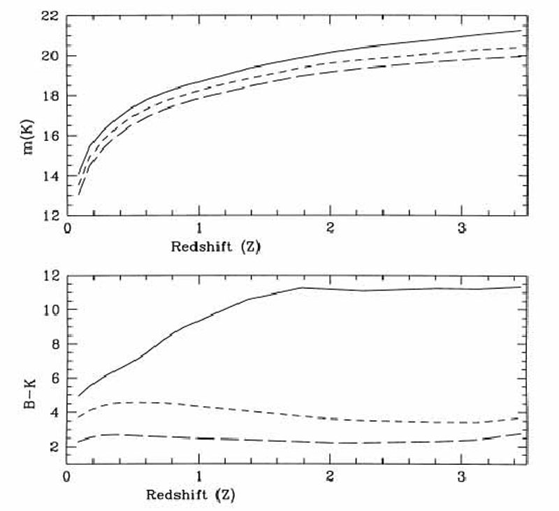Figure 16. The robustness of the K-band luminosity of a galaxy as a proxy for stellar mass (Kauffmann & Charlot 1998). The upper panel shows the K-band apparent magnitude of a galaxy defined to have a fixed stellar mass of 1011 M when placed at various redshifts. The different curves represent extreme variations in the way the stellar population was created. Whereas the B-K color is strongly dependent upon the star formation history, the K-band luminosity is largely independent of it.

In practice the mass/light ratio depends on the assumed distribution of stellar masses in a stellar population. The zero age or initial mass function is usually assumed to be some form of power law which can only be determined reliable for Galactic stellar populations, although constraints are possible for extragalactic populations from colors and nebular line emission (see reviews by Scalo 1986, Kennicutt 1998, Chabrier 2003)

In its most frequently-used form the IMF is quoted in mass fraction per logarithmic mass bin: viz:

or, occasionally,

where x = - 1.

In his classic derivation of the IMF, Salpeter (1955) determined a pure power law with x = 1.35. More recently adopted IMFs are compared in Figure 17. They differ primarily in how to restrict the low mass contribution, but there is also some dispute on the high mass slope (although the Salpeter value is supported by various observations of galaxy colors and H distributions, Kennicutt 1998).

Figure 17. A comparison of popular stellar initial mass functions (courtesy of Ivan Baldry).

The IMF has a direct influence on the assumed M / L_K (as discussed by Baldry & Glazebrook 2003, Chabrier, 2003 and Fukugita & Peebles, 2004) in a manner which depends on the age, composition and past star formation history. The adopted mass/light ratio is then a crucial ingredient for computing both stellar masses (Lecture 4) and galaxy colors.

Baldry ³ has undertaken a very useful comparative study of the impact of various IMF assumptions using the PEGASE 2.0 stellar synthesis code for a population 10 Gyr old with solar metallicity, integrating between stellar masses of 0.1 and 120 M (Table 2). Stellar masses have been defined in various ways as represented by the 3 columns in Table 2. Typically we are interested in the observable stellar mass at a given time (i.e. main sequence and giant branch stars), but it is interesting to also compute the total mass which is not in the interstellar medium, which includes that locked in evolved degenerate objects (white dwarfs and black holes). The most inclusive definition of stellar mass (total) is the integral of the past star formation history. Depending on the definition, and chosen IMF, the uncertainties range almost over a factor of 4 for the most popularly-used functions, quite apart from the unsettling question of whether the form of the IMF might vary with epoch or type of object.

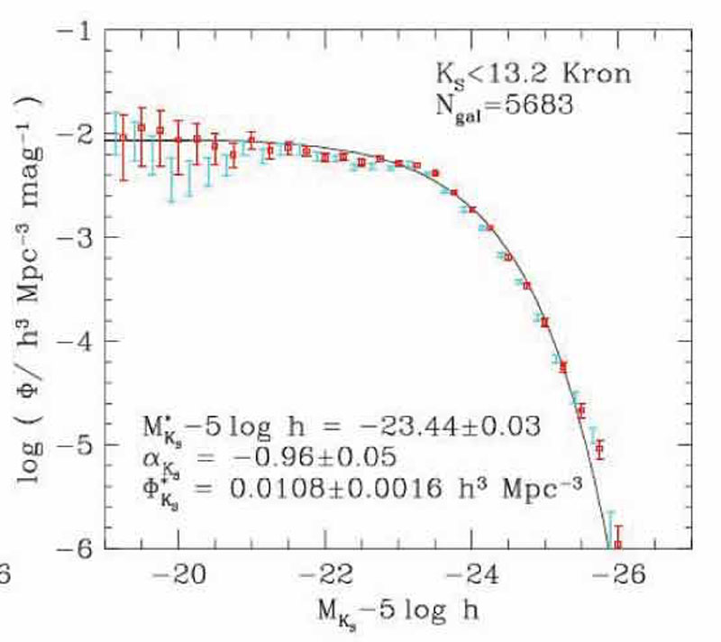
Figure 18 shows the K-band luminosity and derived stellar mass function for galaxies in the 2dF redshift survey from the analysis of Cole et al (2001). K-band measures were obtained by correlation with the K < 13.0 catalog obtained by the 2MASS survey.

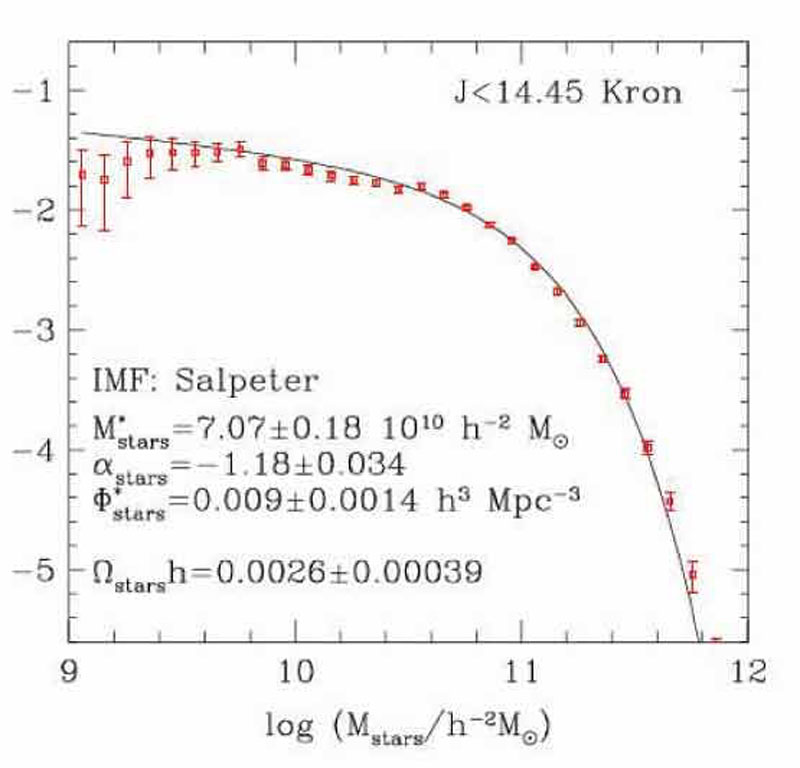Figure 18. (Left) Rest-frame K-band luminosity function derived from the combination of redshifts from the 2dF survey with photometry from 2MASS (Cole et al 2001); Schechter parameter fits are shown. (Right) Derived stellar mass function assuming a Salpeter IMF corrected for lost material assuming R = 0.28 (see text).

The integrated stellar density, corrected for stellar mass loss, is (Cole et al 2001):

for a Salpeter IMF, a value very similar to that derived independently by Fukugita & Peebles (2004). By comparison the local mass fraction in neutral HI + He I gas is:

Thus only 5% of all baryons are in stars with the bulk in ionized gas.

3.3. Diagnostics of Star Formation in Galaxies

When significant redshift surveys became possible at intermediate and high redshift through the advent of multi-object spectrographs, so it became possible to consider various probes of the star formation rate (SFR) at different epochs. As in the formalism for calculating the integrated luminosity density, _L, per comoving Mpc³, so for a given population various diagnostics of on-going star formation can yield an equivalent global star formation rate _SFR in units of M yr^-1 Mpc^-3.

Such integrated measures average over a whole host of important details, such as differences in evolutionary behavior between luminous and sub-luminous galaxies and, of course, morphology. Moreover, in any survey at high redshift, only a portion of the population is rendered visible so uncertain corrections must be made to compare results at different epochs. The importance of the cosmic star formation history, i.e. _SFR(z), is it displays, in a simple manner, the epoch and duration of galaxy growth. By integrating the function, one should recover the present stellar density (Section 3.5).

There are various probes of star formation in galaxies, each with its advantages and drawbacks. Not only is there no single `best' method to gauge the current star formation rate of a chosen galaxy, but as each probe samples the effect of young stars in different initial mass ranges, so each averages the star formation rate over a different time interval. If, as is often the case in the most energetic sources, the star formation is erratic or burst-like, one would not expect different diagnostics to give the same measure of the instantaneous SFR even for the same galaxies.

Four diagnostics are in common use (see review by Kennicutt 1998).

• The rest-frame ultraviolet continuum ( 1250-1500Å) has the advantage of being directly connected to well-understood high mass (> 5M) main sequence stars. Large datasets are available for high redshift star-forming galaxies, including some to z 6. Via the GALEX satellite and earlier balloon-borne experiments, local data is also available. The disadvantage of this diagnostic lies in the uncertain (and significant) corrections necessary for dust extinction and a modest sensitivity to the assumed initial mass function. Obscured populations are completely missed in UV samples. Kennicutt suggests the following calibration for the UV luminosity:

• Nebular emission lines such as H and [O II] are also available for a range of redshifts (z < 2.5), for example as a natural by-product of faint redshift surveys. Gas clouds are photo-ionized by very massive (> 10 M) stars. Dust extinction can often be evaluated from higher order Balmer lines under various radiative assumptions depending on the escape fraction of ionizing photons. The sensitivity to the initial mass function is strong.

• Far infrared emission (10-300 µm) arises from dust heated by young stars. It is clearly only a tracer in the most dusty systems and thus acts as a valuable complementary probe to the UV continuum. As we have seen in Section 2, luminous far infrared galaxies are also seen to high redshift. However, not all dust heating is due to young stars and the bolometric far infrared flux, L_FIR, is needed for an accurate measurement.

• Radio emission, e.g. at 1.4GHz, is thought to arise from synchrotron emission generated by relativistic electrons accelerated by supernova remnants following the rapid evolution of the most massive stars. Its great advantage is that it offers a dust-free measure of the recent SFR. Current radio surveys do not have the sensitivity to see emission beyond z 1, so its promise has yet to be fully explored. This process is also the least well-understood and calibrated. Sullivan et al (2001) discuss this point in some detail and conclude:

  for bursts of duration > 100 Myr.

The question of the time-dependent nature of the SFR is an important point (Sullivan et al 2000, 2001). For an instantaneous burst of star formation, Figure 19a shows the `response' of the various diagnostics. Clearly if the SF is erratic on 0.01-0.1 Gyr timescales, each will provide a different sensitivity. Sullivan et al (2000) compared UV and H diagnostics for a large sample of nearby galaxies and found a scatter beyond that expected from the effects of dust extinction or observational error, presumably from this effect (Figure 19b).

Figure 19. Time dependence of various diagnostics of star formation in galaxies. (Left) sensitivities for a single burst of star formation. (Right) scatter in the UV and H galaxy luminosities in the local survey of Sullivan et al (2000); lines represent model predictions for various (constant) star formation rates and metallicities. It is claimed that some fraction of local galaxies must undergo erratic periods of star formation in order to account for the offset and scatter.

In addition to the initial mass function (already discussed), a key uncertainty affecting the UV diagnostic is the selective dust extinction law. Over the wavelength range 0.3 < < 1 µm, differences between laws deduced for the Milky Way, the Magellan clouds and local starburst galaxies (Calzetti et al 2000) are quite modest. Significant differences occur around the 2200 Å feature (dominant in the Milky Way but absence in Calzetti's formula) and shortward of 2000 Å where the various formulae differ by ± 2 mags in A() / E(B-V).

3.4. Cosmic Star Formation - Observations

Early compilations of the cosmic star formation history followed the field redshift surveys of Lilly et al (1996), Ellis et al (1996) and the abundance of U-band drop outs in the early deep HST data (Madau et al 1996). The pioneering papers in this regard include Lilly et al (1996), Fall et al (1996) and Madau et al (1996, 1998).

Hopkins (2004) and Hopkins & Beacom (2006) have undertaken a valuable recent compilation, standardizing all measures to the same initial mass function, cosmology and extinction law. They have also integrated the various luminosity functions for each diagnostic in a self-consistent manner (except at very high redshift). Accordingly, their articles give us a valuable summary of the state of the art.

Figure 20 summarizes their findings. Although at first sight somewhat confusing, some clear trends are evident including a systematic increase in star formation rate per unit volume out to z 1 which is close to (Hopkins 2004):

A more elaborate formulate is fitted in Hopkins & Beacom (2006).

There is a broad peak somewhere in the region 2 < z < 4 where the UV data is consistently an underestimate and the growing samples of sub-mm galaxies are valuable. The dispersion here is only a factor of ±2 or so, which is a considerable improvement on earlier work. We will return to the question of a possible decline in the cosmic SFR beyond z 3-4 in later sections.

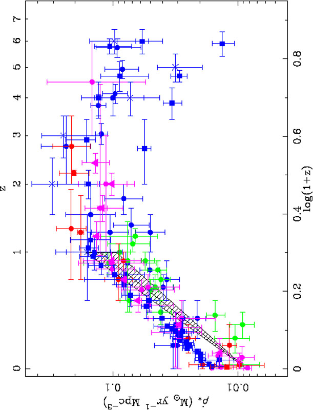Figure 20. Recent compilations of the cosmic star formation history. Circles are data from Hopkins (2004) color-coded by method: blue: UV, green: [O II], red: H / , magenta: non-optical including sub-mm and radio. New data from Hopkins & Beacom (2006), represented by various triangles, stars and squares, include Spitzer FIR measures (magenta triangles). The solid lines represent a range of the best fitting parametric form for z < 1.

In their recent update, Hopkins & Beacom (2006) also parametrically fit the resulting _SFR(z) in two further redshift sections, beyond z 1, and they use this to predict the growth of the absolute stellar mass density, _*, via integration (Figure 21). Concentrating, for now, on the reproduction of the present day mass density (Cole et al 2001), the agreement is remarkably good.

Figure 21. Growth of stellar mass density, *, with redshift obtained by direct integration of a parametric fit to the cosmic star formation history deduced by Hopkins & Beacom (2006, see Figure 20). The integration accurately reproduces the local stellar mass density observed by Cole et al (2001) and suggests half the present density was in place at z = 2.0 ± 0.2.

Although in detail the result depends on an assumed initial mass function and the vexing question of whether extinction might be luminosity-dependent, this is an important result in two respects: firstly, as an absolute comparison it confirms that most of the star formation necessary to explain the presently-observed stellar mass has already been detected through various complementary surveys. Secondly, the study allows us to predict fairly precisely the epoch by which time half the present stellar mass was in place; this is z_1/2 = 2.0 ± 0.2. In Section 4 we will discuss this conclusion further attempting to verify it by measuring stellar masses of distant galaxies directly.

3.5. Cosmic Star Formation - Theory

As we have discussed, semi-analytical models have had a hard time reproducing and predicting the cosmic star formation history. Amusingly, as the data has improved, the models have largely done a `catch-up' job (Baugh et al 1998, 2005a). To their credit, while many observers were still convinced galaxies formed the bulk of their stars in a narrow time interval (the `primeval galaxy' hypothesis), CDM theorists were the first to suggest the extended star formation histories now seen in Figure 20.

A particular challenge seems to be that of reproducing the abundance of energetic sub-mm sources whose star formation rates exceed 100-200 M yr^-1. Baugh et al (2005b) have suggested it may require a combination of quiescent and burst modes of star formation, the former involving an initial mass function steepened towards high mass stars. Although there is much freedom in the semi-analytical models, recent models suggest z_1/2 1.3. By contrast, for the same cosmological models, hydrodynamical simulations (Nagamine et al 2004) predict much earlier star formation, consistent with z_1/2 2.0-2.5.

The flexibility of these models is considerable so my personal view is that not much can be learned from these comparisons either way. It is more instructive to compare galaxy masses at various epochs with theoretical predictions. Although we are still some ways from doing this in a manner that includes both baryonic and dark components, progress is already promising and will be reviewed in Section 4.

3.6. Unifying the Various High Redshift Populations

Integrating the various star-forming populations at high redshift to produce Figure 20 avoids the important question of the physical relevance and roles of the seemingly-diverse categories of high redshift galaxies. In the previous lecture (Section 2), I introduced three broad categories: the Lyman break (LBG), sub-mm and passively-evolving sources (DRGs) which co-exist over 1 < z < 3. What is the relationship between these objects?

As the datasets on each has improved, we have secured important physical variables including masses, star formation rates and ages. We can thus begin to understand not only their relative contributions to the SFR at a given epoch, but the degree of overlap among the various populations. Several recent articles have begun to evaluate the connection between these various categories (Papovich et al 2006, Reddy et al 2005).

A particularly valuable measure is the clustering scale, r₀, for each population, as defined in Section 1.3. This is closely linked to the halo mass according to CDM and thus sets a marker for connecting populations observed at different epochs. Adelberger et al (1998) demonstrated the strong clustering, r₀ 3.8 Mpc, of luminous LBGs at z 3. Baugh et al (1998) claimed this was consistent with the progenitor halos of present-day massive ellipticals. The key to the physical nature of LBGs depends the origin of their intense star formation. At z 3, the bright end of the UV luminosity function is 1.5 mags brighter than its local equivalent; the mean SFR is 45 M yr^-1. Is this due to prolonged activity, consistent with the build up of the bulk of stars which reside in present-day massive ellipticals, or is it a temporary phase due to merger-induced starbursts (Somerville et al 2001).

Shapley et al (2001, 2003) investigated the stellar population and stacked spectra of a large sample of z 3 LBGs and find younger systems with intense SFRs are dustier with weaker Ly emission while outflows (or `superwinds') are present in virtually all (Figure 22a). For the young LBGs, a brief period of elevated star formation seems to coincide with a large dust opacity hinting at a possible overlap with the sub-mm sources. During this rapid phase, gas and dust is depleted by outflows leading to eventually to a longer, more quiescent phase during which time the bulk of the stellar mass is assembled.

If young dusty LBGs with SFRs 300 M yr^-1 represent a transient phase, we might expect sub-mm sources to simply be a yet rarer, more extreme version of the same phenomenon. The key to testing this connection lies in the relative clustering scales of the two populations (Figure 22b). Blain et al (2004) find sub-mm galaxies are indeed more strongly clustered than the average LBGs, albeit with some uncertainty given the much smaller sample size.

Figure 22. Connecting Lyman break and sub-mm sources. (Left) Correlation between the mean age (for a constant SFR) and reddening for a sample of z 3 LBGs from the analysis of Shapley et al (2001). The youngest LGBs seem to occupy a brief dusty phase limited eventually by the effect of powerful galaxy-scale outflows. (Right) The LBG-submm connection can be tested through reliable measures of their relative clustering scales, r0 (Blain et al 2004).

Turning to the passively-evolving sources, although McCarthy (2004) provides a valuable review of the territory, the observational situation is rapidly changing. For many years, CDM theorists predicted a fast decline with redshift in the abundance of red, quiescent sources. Using a large sample of photometrically-selected sources in the COMBO-17 survey, Bell et al (2004) claimed to see this decline in abundance by witnessing a near-constant luminosity density in red sources to z 1 (Figure 23a). The key point to understand here is that a passively-evolving galaxy fades in luminosity so that the red luminosity density should increase with redshift unless the population is growing. Bell et al surmises the abundance of red galaxies was 3 times less at z 1 as predicted in early semi-analytical models (Kauffmann et al 1996).

Figure 23. Left: The rest-frame blue luminosity density of `red sequence' galaxies as a function of redshift from the COMBO-17 analysis of Bell et al (2004). Since such systems should brighten in the past the near-constancy of this density implies 3 times fewer red systems exist at z 1 than locally - as expected by standard CDM models. Right: Composite spectra of red galaxies with 1.3 < z < 1.4 (blue), 1.6 < z < 1.9 (black) from the Gemini Deep Deep Survey (McCarthy et al 2004). A stellar synthesis model with age 2 Gyr is overlaid in red. The analysis suggests the most massive red galaxies with z 5 formed with spectacular SFRs at redshifts z 2.4-3.3.

By contrast, the Gemini Deep Deep Survey (Glazebrook et al 2004) finds numerous examples of massive red galaxies with z > 1 in seeming contradiction with the decline predicted by CDM supported by Bell et al (2004). Of particular significance is the detailed spectroscopic analysis of 20 red galaxies with z 1.5 (McCarthy et al 2004) whose inferred ages are 1.2-2.3 Gyr implying most massive red galaxies formed at least as early as z 2.5-3 with SFRs of order 300-500 M yr^-1. Could the most massive red galaxies at z 1.5 then be the descendants of the sub-mm population? One caveat is that not all the stars whose ages have been determined by McCarthy et al need necessarily have resided in single galaxies at earlier times. The key question relates to the reliability of the abundance of early massive red systems. Using a new color-selection technique, Kong et al (2006) suggest the space density of quiescent systems with stellar mass >10¹¹ M at z 1.5-2 is only 20% of its present value.

As we will see in Section 4, the key to resolving the apparent discrepancy between the declining red luminosity density of Bell et al and the presence of massive red galaxies at z 1-1.5, lies in the mass-dependence of stellar assembly (Treu et al 2005).

Finally, a new color-selection has been proposed to uniformly select all galaxies lying in the strategically-interesting redshift range 1.4 < z < 2.5. Daddi et al (2004) have proposed the `BzK' technique, combining (z-K) and (B-z) to locate both star-forming and passive galaxies with z > 1.4; such systems are termed `sBzK' and `pBzK' galaxies respectively. Reddy et al (2005) claim there is little distinction between the star-forming sBzK and Lyman break galaxies - both contribute similarly to the star formation density over 1.4 < z < 2.6 and the overlap fractions are at least 60-80%.

More interestingly, both Reddy et al (2005) and Kong et al (2006) suggest significant overlap between the passive and actively star-forming populations. Kong et al find the angular clustering is similar and Reddy et al find the stellar mass distributions overlap.

3.7. Lecture Summary

Clearly multi-wavelength data is leading to a revolution in tracking the history of star formation in the Universe. Because of the vagaries of the stellar initial mass function, dust extinction and selection biases, we need multiple probes of star formation in galaxies.

The result of the labors of many groups is a good understanding of the comoving density of star formation since a redshift z 3. Surprisingly, the trends observed can account with reasonable precision for the stellar mass density observed today. The implication of this result is that half the stars we see today were in place by a redshift z 2.

What, then, are we to make of the diversity of galaxies we observe during the redshift range (z 2-3) of maximum growth? Through detailed studies some connections are now being made between both UV-emitting Lyman break galaxies and dust-ridden sub-mm sources.

More confusion reigns in understanding the role and decline with redshift in the contribution of passively-evolving red galaxies. Some observers claim a dramatic decline in their abundance whereas others demonstrate clear evidence for the presence of a significant population of old, massive galaxies at z 1.5. We will return to this enigma in Section 4.

³ http://www.astro.livjm.ac.uk/~ikb/research/imf-use-in-cosmology.html. Back.