2. OBSERVATIONAL EVIDENCE FOR REIONIZATION

To date, the majority of observations related to the EoR provide weak and model dependent constraints on reionization. However, there are currently a number of observations which could impose strong constraints on reionization models, as discussed below. It should be noted however that none of these observations constrains the EoR evolution in detail.

2.1. The Lyman forest at z ≈ 2.5-6.5

The state of the intergalactic medium (IGM) can be studied through the analysis of the Lyman- forest. This is an absorption phenomenon seen in the spectra of background quasi-stellar objects (QSOs). The history of this field goes back to 1965 when a number of authors [74, 179] predicted that an expanding Universe, homogeneously filled with gas, will produce an absorption trough due to neutral hydrogen, known as the Gunn-Peterson trough, in the spectra of distant QSOs bluewards of the Lyman- emission line of the quasar. That is, the quasar flux will be absorbed at the UV resonance line frequency of 1215.67 Å. Gunn & Peterson [74] found such a spectral region of reduced flux, and used this measurement to put upper limits on the amount of intergalactic neutral hydrogen. The large cross-section for the Lyman absorption makes this technique very powerful for studying gas in the intergalactic medium.

In the last 15 years two major advances occurred. The first was the development of high-resolution echelle spectrographs on large telescopes (e.g., HIRES on the Keck and UVES on the Very Large Telescope) that provided data of unprecedented quality. The second was the emergence of a theoretical paradigm within the context of cold dark matter (CDM) cosmology that accounts for all the features seen in these systems (e.g. [16, 39, 81, 118, 131, 201, 232, 233]). According to this paradigm, the absorption is produced by volume filling photoionized gas that contains most of the baryons at redshifts at z ~ 3-6 and resides in mildly non-linear overdensities.

Figure 3 shows a typical example of the Lyman forest seen in the spectrum of the z = 3.12 quasar Q0420-388. An interesting feature of such spectra is the density of weak absorbing lines which increase with redshift due to the expansion of the Universe. In fact, at redshifts above 4, the density of the absorption features become so high that it is hard to define them as separate absorption features. Instead, one sees only the flux in between the absorption minima which appears as if they are emission rather than absorption lines.

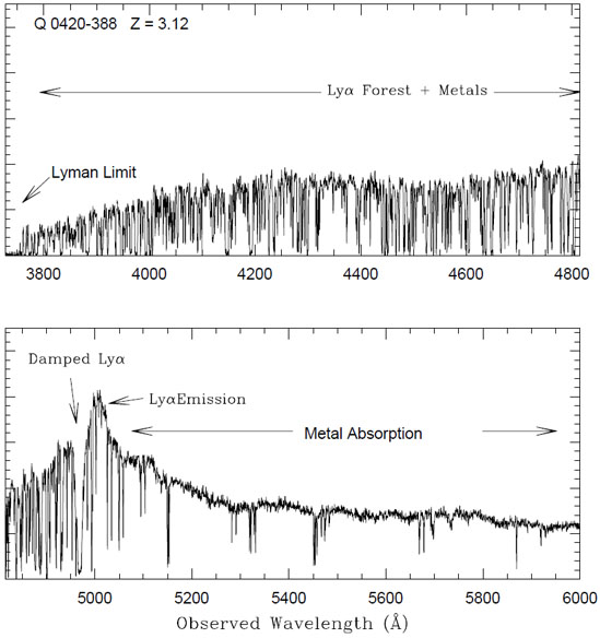Figure 3. High resolution spectrum of the z = 3.12 quasar Q0420-388 obtained with the Las Campanas echelle spectrograph by J. Bechtold and S. A. Shectman. The two panels cover the whole wavelength range of the spectrum. The Lyman forest is clearly indicated in the upper panel of the figure, bluewards of the quasar rest frame Lyman emission feature. Remember, at the rest frame this feature should have a wavelength of 1215.67 Å but since it is redshifted by a factor 1 + z it appears at a wavelength of about 5000 Å. The Figure is courtesy of Jill Bechtold and appeared in [11].

The Lyman forest has turned out to be a treasure trove for studying the intergalactic medium and its properties in both low and high density regions. In particular, it is very sensitive to the neutral hydrogen column density and hence, to the neutral fraction as a function of redshift along the line of sight. In the following, we demonstrate how one could constrain the neutral fraction of hydrogen from the forest and what the values obtained from the data are. For a review on the Lyman forest the reader is referred to [162].

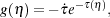
We need to calculate the optical depth for absorption of Lyman photons. A photon emitted by a distant quasar with an energy higher than 10.196 eV is continuously redshifted as it travels through the intergalactic medium until it reaches the observer. At some intermediate point the photon is redshifted to around 1216 Å in the rest-frame of the intervening medium, which may contain neutral hydrogen. It can then excite the Lyman transition and be absorbed. Let us consider a particular line of sight from the observer to the quasar. The optical depth of a photon is related to the probability of the photon's transmission e^-. At a given observed frequency, ₀, the Lyman optical depth is given by

(1)

where l is the comoving radial coordinate of some intermediate point along the line of sight, z is the redshift and n_HI is the proper number density of neutral hydrogen at that point. The limits of the integration, O and Q, are the comoving distance between the observer and the quasar, respectively. The Lyman absorption cross section is denoted by . It is a function of the frequency of the photon, , with respect to the rest-frame of the intervening H I at position l. The cross section is peaked when is equal to the Lyman frequency . The frequency is related to the observed frequency ₀ by = ₀(1 + z), where 1 + z is the redshift factor due to the uniform Hubble expansion alone at the same position. Note that for the sake of simplicity here we ignore peculiar velocity effects.

Using dl = c dt / a, where a is the Hubble scale factor and t is the proper time and Friedmann equation for a flat Universe with cosmological constant, we have,

(2)

This optical depth should also depend on the Lyman line profile function but here we assume that it is basically a -function centered at the frequency . Considering n_HI = n_H x_HI, where x_HI is the neutral fraction of hydrogen, and integrating over this equation, one obtains the following result:

(3)

Since the Lyman features mostly show mild absorption probability ( 1) this equation clearly implies that at the mean density of the Universe at of about one the ionized fraction is on the order of 10^-4. Therefore, the fact that we observe the Lyman forest at all means that the Universe is highly ionized at least until z ≈ 6. This is the most reliable and robust evidence that the Universe has in fact reionized.

Another important evidence relevant for reionization comes from high resolution spectroscopy of high redshift Sloan Digital Sky Survey (SDSS) quasars [59, 60]. The SDSS has discovered about 19 QSOs with redshifts around 6 that are powered by black holes with masses on the order of 10⁹ M. In a follow up observations with 10 meter class telescopes Fan et al. [59, 60] were able to obtain high resolution spectra of these objects.

Fig. 4 shows the spectra of these high redshift quasars [59, 60]. Notice the complete absence of structure that some of these spectra exhibit bluewards of the quasar Lyman restframe emission, especially those with redshift z 6. This is normally attributed to an increase in as a result of the decrease in the ionized fraction of the Universe. Notice also, that although the trend with redshift is clear, it is by no means monotonic. For example, quasar J1411+3533 at z = 5.93 shows an "emptier" trough relative to quasars J0818+1722 at z = 6. Such trend might be indicating a more patchy ionization of the IGM at such redshifts.

Figure 4. Spectra for high redshift SDSS quasars. The Gunn-Peterson trough bluewards of the QSO Lyman emission that is clearly apparent in the highest redshift ones indicates that the Universe has become somewhat more neutral at these redshifts. A similar behavior is also seen bluewards of the QSO Lyman region of the same spectra. The actual amount of increase in neutral hydrogen implied by these spectra is not clear [60].

Figure 5 shows the effective Lyman or Gunn-Peterson optical depth, _GP^eff, as a function of redshift as estimated from the joint optical depths of Lyman , and . From this plot it is clear that the increase in the optical depth as a function of redshift is much larger than expected (shown in the dashed line) from passive redshift evolution of the density of the Universe.

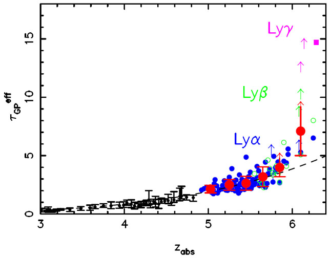Figure 5. Evolution of the Lyman , and optical depth from the high redshift Sloan quasars. The Lyman and Lyman restframe wavelengths are 1026 Å and 972.5 Å, respectively. The Lyman measurements are converted to Lyman Gunn-Peterson optical depth using a conversion factor that reflects the difference in the cross section between the two transitions, which is a factor of 5.27 lower in the case of Lyman (see [112, 38]) . The values in the two highest redshift bins are lower limits, since they both contain complete Gunn-Peterson troughs. The dashed line shows a redshift evolution of ≈ (1 + z)4.3. At z > 5.5, the best-fit evolution has ≈ (1 + z)> 10.9, indicating an accelerated evolution. The large filled symbols with error bars are the average and standard deviation of the optical depth at each redshift. The sample variance also increases rapidly with redshift. Figure taken from [60].

The interpretation of the increase in the optical depth at z 6.3 has been the subject of some debate. All authors agree that this is a sign of an increase in the Universe's neutral fraction at high redshifts, marking the tail end of the reionization process. The controversy is centered on the question of by how much the neutral fraction increases. Some authors [217, 218, 130] have argued that the size of the so call Near Zone ionized by the quasar itself and set redwards of the Gunn-Peterson trough indicates that the neutral fraction around the SDSS high redshift quasars is ≈ 10%. More recently is had been suggested that the variations seen across various SDSS quasars indicate that the ionization state of the IGM at these redshifts changes significantly across different sightlines [128]. However, given the intense radiation field around these quasars, it is not possible to put general constraints on the neutral fraction of the IGM from quasars at redshift below 6.5 (see e.g., [18, 216, 123, 124]). Moreover, recently and with the discovery of the redshift z = 7.1 QSO ULAS J1120+0641 [137] by the UKIDSS survey [108] it has been argued that this quasar's Near Zone gives a clear evidence for an increase in the neutral fraction of hydrogen in the IGM at z = 7.1 [137, 20]. Note however that his conclusion relies on one quasar and might change as more of such quasars at z 7 are discovered.

There are more things that we can learn about reioinzation from the Lyman forest that we will discuss later. But to summarize, the main conclusion from the Lyman optical depth measurements is that the Universe is highly ionized at redshifts below 6 (as seen in Figure 4), while at about z = 6.3, the its neutral fraction increases, forming the tail end of the reionization process (see Figure 5) .

2.2. The Thomson Scattering Optical depth for the Cosmic Microwave Background (CMB) Radiation

This is a very evolved topic, discussed and reviewed by many authors (e.g., [157, 195, 21, 117, 86, 4]). Here, I give a general review of the constraints provided by the CMB on reionization. The CMB provides important information relevant to the history of reionization. It is known that the Universe has indeed recombined and became largely neutral at z ≈ 1100. If recombination had been absent or substantially incomplete, the resulting high density of free electrons would imply that photons could not escape Thomson scattering until the density of the Universe dropped much further. This scattering would inevitably destroy the correlations at subhorizon angular scales seen in the CMB data (see e.g., [85, 190]).

In order to calculate the effect of reionization on CMB photons, a function is often defined called the visibility function ¹,

(4)

where (≡ ∫ dt / a ) is the conformal time, a is the scale factor of the Universe and is the derivative of the optical depth with respect to to . The optical depth for Thomson scattering is given by () = -∫^₀ d = ∫^₀ d a() n_{e T}, where ₀ is the present time, n_e is the electron density and _T is the Thomson cross section. The visibility function gives the probability density that a photon had scattered out of the line of sight between and + d. The influence of reionization on the CMB temperature fluctuations is obtained by integrating Equation 4 along each sightline to estimate the temperature fluctuation suppression due to the EoR. The suppression probability turns out to be roughly proportional to 1 - e^- [224]. Since the amount of suppression in the measured power spectrum is small, the optical depth for Thomson scattering must be small too [152]. The left hand panel in Figure 6 shows the influence of increasing the value of , the Thomson optical depth, on the CMB temperature fluctuation power spectrum. The right hand panel shows the reionization history of the Universe assumed in the left panel. Since in this case a sudden global reionization is assumed, there is one to one correspondence between the optical depth for Thomson scattering and the redshift of reionization.

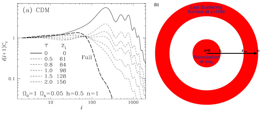Figure 6. Left hand panel (a): The influence of reionization on the CMB temperature angular power spectrum. Reionization damps anisotropy power as e-2 under the horizon (diffusion length) at last scattering. The models here are fully ionized xe = 1.0 out to a reionization redshift zi. Notice that with high optical depth, fluctuations at intermediate scales are regenerated as the fully ionized (long-dashed) model shows. This figure is taken from Wayne Hu's PhD thesis [85]. Right panel (b) shows the assumed reionization history used. It is obvious that since we are considering a uniform and sudden reionization model, a change in the reionization redshift, zi, will translate uniquely to an optical depth for Thomson scattering.

Further information can be obtained from observations of CMB via the polarization power spectrum. The polarization of the CMB emerges naturally from the Cold Dark Matter paradigm which stipulates that small fluctuations in the early universe grow, through gravitational instability, into the large scale structure we see today ([21, 86, 97, 227]). Since, the temperature anisotropies observed in the CMB are the result of primordial fluctuations, they would naturally polarize the CMB anisotropies. The degree of linear polarization of the CMB photons at any scale reflects the quadrupole anisotropy in the plasma when they last scattered at that same scales. From this argument it is clear that the amount of polarization at scales larger than the horizon scale at the last scattering surface should fall down since there is no more coherent quadrupole contribution due to the lack of causality. This is shown in the sketch presented in the left hand panel in Figure 7. The largest scale at which a primordial quadrupole exists is the scale of the horizon at recombination, which roughly corresponds to 1°. Therefore, any polarization signature on scales larger than the horizon scale provides a clear evidence for Thomson scattering at later stages where the horizon scale is equivalent to the scale on which polarization has been detected.

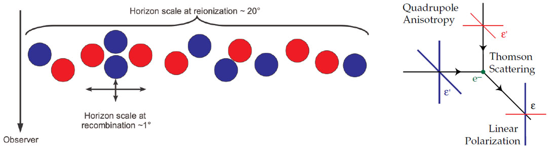Figure 7. Left hand panel: A sketch that shows why the CMB polarization is sensitive to the quadrupole momentum of temperature fluctuations. Right hand panel: Thomson scattering of radiation with quadrupole anisotropy generates linear polarization. The blue and red lines represent cold and hot radiation.

Furthermore, the polarized fraction of the temperature anisotropy must be small, normally one order of magnitude smaller than the anisotropy in the temperature. This is simply because these photons mush have passed through an optically thin plasma, otherwise they would not have reached us but they would have scattered and destroyed the sub-horizon (i.e., below 1°) correlation in the CMB, contrary to what we observe (see e.g., [190]).

The dependence Thomson scattering differential cross section on polarization is expressed as

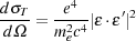(5)

where e and m_e are the electron charge and mass and є ⋅ є' is the angle between the incident and scattered photons. The right hand panel of Figure 7 shows how the Thomson scattering produces polarization of the CMB photons. If the CMB photons scatter later due to reionization and the incident radiation has a quadrupole moment, then it will be scattered in a polarized manner on the scale roughly equivalent to the horizon scale at the redshift of scattering. That is why the scale at which the large scale polarization is detected gives information about the reionization redshift.

The polarization field of the CMB photons is usually described in terms of the so called "electric" (E) and "magnetic" (B) components which can be derived from a scalar or vector field. The harmonics of an E-mode have (-1)^ℓ parity on the sphere, whereas those of B-mode have (-1)^ℓ+1 parity. Under parity transformation, i.e., n → - n, the E-mode thus remains unchanged for even ℓ , whereas the B-mode changes sign and vice versa. Fig. 8 illustrates such (a)symmetry under parity transformation for the simple case of ℓ = 2, m = 0 [86].

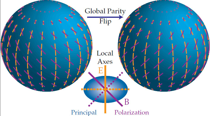Figure 8. The E and B polarization modes are distinguished by their behavior under parity transformation. The local distinction is that the E mode is aligned with the principle axis of polarization whereas the B mode is 45° crossed with it (this figure is taken from Hu and White [86]).

Various physical processes lead to different effects on the CMB polarization. Most of these effects are expected to produce E mode polarization patterns on the CMB. However, gravitational waves in the primordial signal and gravitational lensing of the CMB on its way to us produce a B mode polarization patterns. A large scale E mode polarization signal could only be caused by the process of reionization. The main reason for this is that large scale polarization could not be caused by causal effects on the last scattering surface which has a 1° scale whereas reionization, which occurs much later, has no such restriction. Figure 9 shows the measured and predicted CMB angular power and cross-power spectra from the WMAP 3^rd year data. The existence of large scale correlation in the E-mode is a strong indication that the Universe became ionized around redshift z ≈ 10. The argument in essence is mostly geometric, namely it has to do with the scale of the E-mode power spectrum as well as the line of sight distance to the onset of the reionization front along a given direction. Some authors have also argued that one can have somewhat more detailed constraints on reionization from the exact shape of the CMB E-mode polarization large scale bump [84, 110, 138]. Unfortunately however, the large cosmic variance at large scales limits the amount of possible information one can extract. Still, the Planck surveyor is expected to be able to retrieve some of the large scale bump shape.

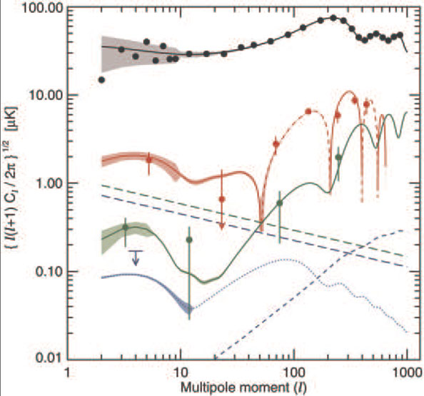Figure 9. The temperature and E-mode polarization power and cross-power spectra as measure by the WMAP satellite [152]. Plots of signal for TT (black), TE (red ), and EE ( green) for the best-fit model. The dashed line for TE indicates areas of anticorrelation. For more details about this Figure we refer the reader to the Page et al. [152]. Notice the excess power on large scales caused by reionization seen in the TE and EE power spectra.

From Figure 9 one can also deduce the optical depth for Thomson scattering, , caused by the scattering of the CMB photons off free electrons released by reionization to be 0.087 ± 0.017 [57]. This could be turned into a constraint on the global reionization history through the integral,

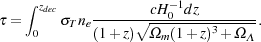(6)

Here z_dec is the decoupling redshift, _T is the Thomson cross section, µ is the mean molecular weight and n_e is the electron density. This formula works for the optical depth along each sight line but also for the mean electron density, i.e., mean reionization history, of the Universe.

An important point to notice here is that, in order to turn into a measurement of the reionization redshift, one needs a model for n_e as a function of redshift. Hence, one has to be careful when using the reionization redshift given by CMB papers as in most cases a gradual reionization is assumed. Sudden reionization gives a one to one correspondence between the measured optical depth and the reionization redshift, e.g., the WMAP measurement optical depth implied z_i = 11.0 ± 1.4.

However, sudden reionization is very unlikely and most models predict a more gradual evolution of the electron density as a function of redshift. Furthermore, in such scenarios the redshift of reionization is not clearly defined, therefore authors refer instead to the redshift at which half of the IGM volume is ionized, z_{xHI = 0.5}. Obviously, in the case of sudden reionization the two redshifts coincide, z_i = z_{xHI = 0.5}. It is also important to notice that in the case of sudden reionization the WMAP measured Thomson optical depth does not imply that the redshift at which half the IGM is ionized is the same as z_i and in most cases one obtains z_{xHI = 0.5} < z_i [206].

The patchy nature of the reionization process will also leave an imprint at arcminute scales on the CMB sky. Such an imprint will be mostly caused by the reionization bubbles that form during the EoR. However, the strength of the reionization signal at small scales is found to be smaller than that caused by gravitation lensing and is very hard to extract unless the experiment has a very high signal-to-noise at such small scales [54].

2.3. The Intergalactic Medium at z 6

There are a number of other observations that put somewhat less certain constraints on reionization. Those constraints come mostly from detailed analysis of high resolution Lyman forest data and from the observation of high redshift Lyman break galaxies. Here we present the two "strongest" of those constraints.

2.3.1. IGM Temperature Evolution

Another constraint on the reionization history comes from studying the thermal history of the IGM. Due to its low density, the intergalactic medium cooling time is long and retains some memory of when and how it was last heated, namely, reionized. Hence, measuring the IGM temperature at a certain redshift ( 3.5) allows us to reconstruct, under certain assumptions, its thermal history up to the reionization phase where the IGM has been substantially heated. Such a measurement has been carried out by a number of authors using high resolution Lyman forest data, especially using the very low column density absorption lines. The width of these absorption features carries information about the temperature of the underlying IGM. This temperature obviously varies with density and with other parameters like the background UV flux. Based on both theoretical arguments [87] and on numerical simulations [201] in the linear and quasilinear regime, the temperature-density relation follows the simple power law,

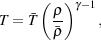(7)

where is the temperature of the IGM at the mean density of the Universe and is the adiabatic power law index. Figure 10 shows the so called phase diagram, i.e., the relation between the temperature and density, obtained from a cosmological hydrodynamical simulation [161]. The relation between the density and temperature at the low density end of the diagram, marked as diffuse background, follows a power law. The hot phase at intermediate densities where cooling is not efficient, is driven by shock heating. At high densities, cooling becomes very efficient and drives the gas temperature. At high redshifts more than 90% of the gas is in the diffuse phase.

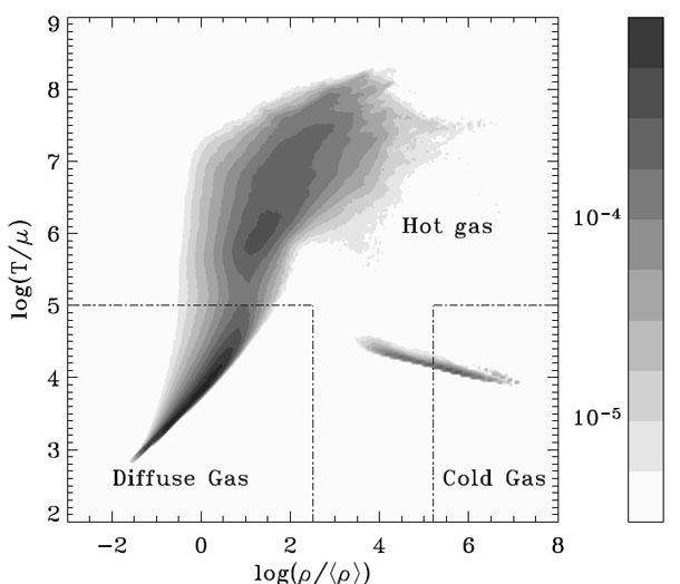Figure 10. The different baryon phases in the - T diagram. Gray contours show a mass-weighted histogram: the baryon mass fraction at a given density and temperature. Each region corresponds to a given phase (diffuse background, hot, or cold gas) [161].

Given the validity of equation 7 at low densities, it is meaningful to define an IGM temperature as the gas temperature at the mean density, . Such a measurement has been performed by a number of authors at z ≈ 3-4 [111, 178, 203, 225] and recently at z ≈ 6 by [17].

The usefulness of this temperature to constrain the reionization history was first realized by [202, 88] who used the measured temperature around redshift 3 to set z ≈ 9 as an upper limit for the reionization process. Bolton et al. ([17]) have recently confirmed these findings with higher redshift quasars. That is, the measured temperatures of the IGM at redshift z ≈ 3 and z ≈ 6 are too high for the bulk of reionization to have occurred at redshift 10.

After reionization, the evolution of the IGM mean temperature is given by

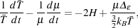(8)

where H is the Hubble parameter, k_B is the Boltzmann constant, µ is the mean molecular weight, and _є is the effective radiative cooling rate (in units of ergs g^-1 s^-1). _є is negative (positive) for net cooling (heating) and includes photoelectric heating and cooling via recombination, excitation, inverse Compton scattering, collisional ionization, and bremsstrahlung. Without cooling/heating processes the cooling rate is set by adiabatic cooling, namely, Hubble expansion. This equation enables us to calculate the temperature evolution as a function of redshift. Measuring the IGM temperature at a given redshift will allow us to extrapolate back in time until we reach a temperature of 6 × 10⁴ K which is the temperature at which hydrogen ionizes. Figure 11 demonstrates this procedure [202].

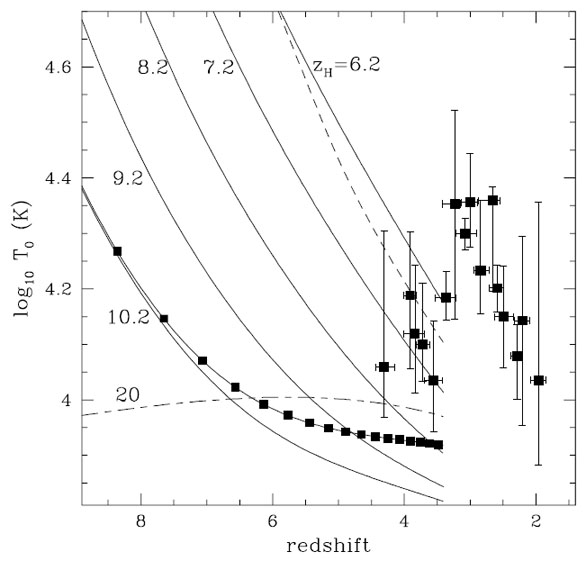Figure 11. Temperature evolution of the IGM above redshift 3.4. The solid curves indicate the evolution of the temperature at the mean density for various H I reionization redshifts zH, as indicated. The temperature after hydrogen reionization is assumed to be T0 = 6 × 104 K, and the hydrogen photoionization rate is = 10-13 s-1 ( = 10-14 s-1, short-dashed curve). The He IIphotoionization rate is adjusted so that the He III abundance is xHeIII ≈ 0.1 at z = 3.5. The solid curve connecting the filled squares indicates zH = 10.2 and a higher He II photoionization rate, xHeIII(z = 3.5) = 0.6. Finally, the long-dashed curves has zH = 20 but a still higher He II photoionization rate, xHeIII(z = 3.5) = 0.95. If He is mostly singly ionized at z ≈ 3.5, then the rapid decrease in T0 after reionization places an upper limit of zH < 9 on the redshift of hydrogen reionization. The filled squares with error bars show the measured IGM temperature as as function of redshift. This figure taken from [202].

2.3.2. Number of Ionizing Photons per Baryon

Another constraint that comes mostly from the Lyman forest but also from the recently discovered galaxies at z 7 is the number of ionizing photons per baryon. Using physically motivated assumptions for the mean free path of ionizing photons, Bolton and Haehnelt ([18]) turned the measurement of the photoionization rate into an estimate of the ionizing emissivity. They showed that the inferred ionizing emissivity in comoving units, is nearly constant over the redshift range 2-6 and corresponds to 1.5-3 photons emitted per hydrogen atom over a time interval corresponding to the age of the Universe at z = 6. Completion of reionization at or before z = 6 requires therefore, either an emissivity which rises towards higher redshifts or one which remains constant but is dominated by sources with a rather hard spectral index, e.g., mini-quasars.

With the installation of the WFC3 camera aboard the Hubble Space Telescope, searches for high redshift galaxies at z = 6-10 have improved dramatically. In particular, a number of authors [145, 23, 33, 125] have reported detection of very high redshifts galaxies using the Lyman-break drop-out technique. The most striking result of these studies is the low number of galaxies found beyond redshift ≈ 6, making it very hard for these galaxies to ionize the Universe. This conclusion depends however on assuming a luminosity function for galaxies at these redshifts, a function that is very poorly known. More surprising is the very steep drop in the number of galaxies at redshift z ≈ 9 [22] which makes it even harder to explain reionization with such galaxies.

The last two observational findings have led some authors to claim that the reionization is photon starved, i.e., has a low number of ionizing photons per baryon, which results in a very slow and extended reionization process [18, 34]. Figure 12 shows the number density of ionizing photons (left-hand vertical axis) and number of ionizing photons per baryon (right-hand vertical axis) as a function of redshift. The number of ionizing photons per baryon at redshift 6 is of the order of 2. More recent results deduced from Lyman-break galaxies are consistent with this figure and show an even lower ratio of ionizing photons per baryon at higher redshifts.

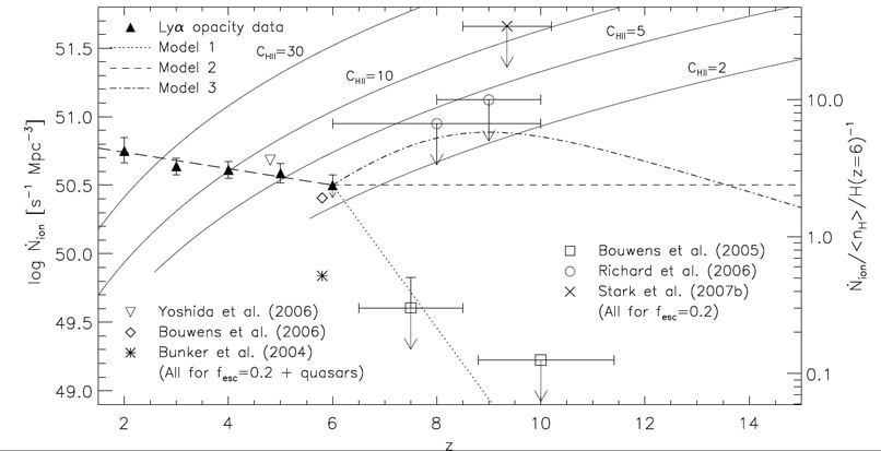Figure 12. Observational constraints on the emission rate of ionizing photons per comoving Mpc, ion, as a function of redshift. The scale on the right-hand vertical axis corresponds to the number of ionizing photons emitted per hydrogen atom over the Hubble time at z = 6. The filled triangles give an estimate of ion based on the constraints obtained from the Lyman effective optical depth from [19] . The inverted triangle at z = 5 and the diamond and star at z = 6 correspond to estimates of ion based on the Lyman limit emissivities of LBGs and quasars. The data have been slightly offset from their actual redshifts for clarity. An escape fraction of fesc = 0.2 has been assumed in this instance. At z > 6, the open squares and circles are derived from the upper limits on the comoving star formation rate per unit volume inferred by [24, 164], respectively. The cross is derived from the number density of Lyman emitters estimated by [188]. Three simple models for the evolution of ion are also shown as the dotted, short dashed and dot-dashed lines. The solid lines correspond to the emission rate of ionizing photons per unit comoving volume, rec, needed to keep the IGM ionized for various H II clumping factors. This figure is taken from [18], see also [34].

2.4. Other Observational Probes

In addition to the probes that we discussed so far, there are a large number of other observational probes that could potentially add valuable input to the reionization models. Examples of such probes are cosmic infrared and soft x-ray backgrounds [52], Lyman emitters [149], high redshift QSOs [137] and GRBs [31], metal abundance at high redshift [172], etc. However, such probes currently provide very limited constraints on the EoR.

In the coming chapters we will focus on the very large effort currently made to measure the diffuse neutral hydrogen in the IGM as a function of redshift up to z 11 using the redshifted 21 cm emission line. This probe will give the most direct and detailed evidence on the reionization process.

¹ Notice that this is a different "visibility" than the one used in radio interferometry which we discuss in section 5. Back.