


Type IIP SNe can be used as "standardized" candles to estimate distances well within the Hubble flow, with a rms precision of the order of 10−15 %. This occurence makes them interesting cosmological distance indicators, since they are produced by different stellar populations than type Ia SNe, making them useful sanity check of the type Ia SNe-based results. More generally, it has demonstrated that all type II (IIP + IIL) SNe can be used as standardized candles (e.g., de Jaeger et al, 2015, 2017). Here the current status of the type IIP SNe standardized candle method is reviewed, pointing out the need for a calibration based on primary distance indicators.
In the classical classification scheme (Filippenko 1997b), type IIP SNe are characterized spectroscopically by strong hydrogen emission features, with strong P-Cygni profiles; and photometrically by a long plateau, lasting on average ∼ 80 days, followed by a sudden drop in luminosity and a subsequent settlement on the radioactive tail.
From the physical point of view, both theoretical (e.g., Grassberg et al, 1971, Litvinova and Nadezhin 1983, Utrobin and Chugai 2008, Pumo and Zampieri 2011) and empirical investigations (e.g., Smartt et al, 2009) show that type IIP SNe are the product of a core collapse of a small to moderate massive progenitors, typically red supergiants (RSG). Interestingly, while on the basis of the empirical models (Heger et al, 2003, Walmswell and Eldridge 2012) we expect that type IIP SNe are the final fate of progenitors of masses between 8 M⊙ and 30 M⊙, empirical evidence found progenitors only in the range 8−17 M⊙. This discrepancy has been dubbed the "RSG problem" (Smartt 2009). However, some claims in the recent literature suggest higher mass limits (e.g., Dall'Ora et al, 2014), while independent studies of the massive star populations in the Local Group found RSGs with masses up to ∼ 25 M⊙ (Massey et al, 2000, 2001).
The characteristic photometric plateau is supported by the hydrogen recombination front, which recedes in mass as the photosphere expands and cools down, producing a constant luminosity. As the density lowers down to values in correspondence of which the atmosphere becomes transparent, a sudden drop ( ∼ 30 days) in luminosity of several magnitudes is observed, and the light curve is subsequently powered only by the radioactive decay of 56Co to 56Fe. In this phase, the SN luminosity depends on the amount of 56Ni synthesized in the explosion (e.g., Weaver and Woosley 1980).
Since type IIP SNe are produced by a variety of progenitors, with different masses and chemical compositions, the observed features (luminosity at the plateau, length of the plateau, kinetic energy of the ejecta, amount of synthesized 56Ni) can be very different from SN to SN (see Fig. 5, from Anderson et al, 2014 here reproduced by kind permission). Indeed, absolute plateau magnitudes range typically from MV = −15.5 mag to MV = −18.5 mag, initial velocity of the ejecta are of the order of 1−2 × 10⁴ km sec−1, and initial photospheric temperatures are of usually around 1−2 × 10⁴ K.
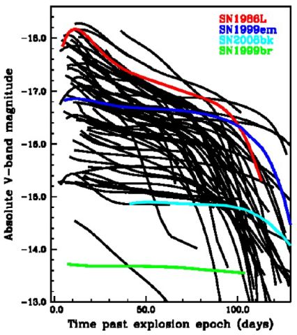 |
Figure 5. Absolute V-band magnitudes of a sample of 60 type IIP SNe, as published in Anderson et al (2014). Reproduced by kind permission of the authors. |
Nevertheless, interestingly and physically motivated relationships between observable quantities, such as between the linear radius (estimated from the velocity curve) and the angular radius (estimated by fitting a black body to the observed fluxes at different epochs); or between the luminosity at the middle plateau and expansion velocity, allow us to use them as "standardized" distance indicators. The first method is known as the expanding photosphere method (EPM, Kirshner and Kwan 1974), while the second has been dubbed the "standardized candle method" (SCM, Hamuy and Pinto 2002). Quite interestingly, the two methods can give consistent results, up to cosmological distances (e.g. Gall et al, 2016).
3.2. Physical basis of the EPM and SCM method
EPM is actually a variant of the Baade-Wesselink method, able to produce very accurate results (see Bose and Kumar 2014). The method requires the measurement of the temperature of the expanding stellar envelope, and of the envelope radius, which in turn comes from measurement of time since explosion and the expansion speed from the Doppler shift of the lines. Thus, it allows to measure the absolute luminosity, and finally to obtain the luminosity distance in a direct way. Type II SNe are intrinsicaly bright, so this method is able to provide distance estimates up to cosmological distances, independently from the adopted distance ladder, thus providing an independent check of the results obtained, for example, with the type Ia SNe, and it can be applied at any phase. However, it is observationally demanding, since it requires multi-band photometric data and good quality spectra. Moreover, some modeling is needed, especially in correctly estimating the dilution factor of SNe atmospheric models respect to a pure black body. A further improvement of the EPM is the spectral fitting expanding atmosphere method (SEAM, Mitchell et al, 2002), based on full NLTE atmospheric code. It can give quite accurate and precise results (e.g. Baron et al. 2004, Bose and Kumar 2014), but it is computationally intensive and requires high S/N spectra at early phases.
SCM was introduced by Hamuy & Pinto in 2002 (Hamuy and Pinto 2002, hereafter HP02) as an empirical correlation between the SN luminosity and the expansion velocity of the ejecta. They calibrated their luminosity-velocity relation at day 50 in the V and I photometric bands, which corresponds to a middle-plateau phase for most of the type IIP SNe. Subsequently, Kasen and Woosley (2009) provided theoretical basis on the SCM. As a matter of fact, SCM is a simple recasting of the Baade-Wesselink method. Indeed, since the expansion is homologous (and therefore the velocity is proportional to the radius), the luminosity L can be written as L = 4 πv2ph t2 ζ2 T4ph, where vph and Tph are the photospheric velocity and temperature, respectively; ζ is a dilution factor, which accounts for the departure from a perfect blackbody, while t is the reference epoch. Now, t can be arbitrarily chosen (50 day by construction), and Tph is a good proxy of the temperature TH of the hydrogen recombination, Th ≈ 6000K, nearly a constant along the plateau. Finally, the dilution factor ζ can be estimated from NLTE models, but it is a strong function of the luminosity, and it can be absorbed in the exponent. It should be explicitly noted that SCM does not need to be applied necessarily at day 50, and that similar relations are valid all along the plateau. However, at epochs earlier than day 30 the ejecta temperature is too high, and probably the approximation Tph ∼ Th is not valid. Moreover, the atmospheric velocity curve is rapidly changing during the first 40−50 days, and a 10−15 days uncertainty in the explosion epoch can reflect in a substantial bias in the velocity curve.
3.3. Current calibrations: an overview
The first calibration was given by HP02 that, on the basis of 17 literature type IIP SNe, 8 of which well embedded in the Hubble flow, derived a relation in the V and the I band as a function of the photospheric velocity and of the redshift. Their calibration showed a scatter of the order of 9%, comparable with the precision of 7%, typical of type Ia SNe. However, an estimate of the absorption is needed, and this is usually a thorny problem when dealing with SNe. The problem was faced by Hamuy (2003), where the absorption was estimated on the basis of observed (V − I) colors. Indeed, when it is assumed that the intrinsic end-of-the-plateau (V − I) color is the same for all the type IIP SNe and it is a function of the photospheric temperature only, a possible (V − I) color excess is due to the host galaxy extinction. The underlying physical assumption is that in type IIP SNe the opacity is mainly caused by the e− scattering, so that they reach the same hydrogen recombination temperature as they evolve. However, some discrepancies are obtained, probably due to metallicity variations from one SN to the other. Moreover, as pointed out by Nugent et al. (2006), a color-based extinction correction is impractical for faint (i.e. basically distant) SNe, since it would require a continuous monitoring to catch the end of the plateau, before the luminosity drop.
A subsequent calibration was then proposed in 2006 by Nugent et al (2006) (N06), where an extinction correction was determined from the rest-frame (V − I) color at day 50, adopting a color-stretch relationship, as done in Ia SNe studies. A standard RV = 3.1 dust law was used. Moreover, since at moderate redshifts the weak Fe II λ5169 could be hardly measured (because they can be redshifted into the OH forest), they explored the practicality of stronger lines, such as the Hβ. Also, they derived an useful empirical relation to scale the observed Fe II λ5169 velocity at a given epoch, to the reference +50 day. They obtained the first Hubble diagram at cosmologically relevant redshifts (z ∼ 0.3) with a rms scatter in distance of 13 %, which is comparable with the rms scatter obtained with Ia SNe.
Poznanski and coworkers (Poznanski et al, 2009, hereafter P09) used a fitting method similar to those adopted by N06, but taking the extinction law as a free paramenter. This procedure yielded a mild total-to-selective absorption ratio RV = 1.5 and, after discarding a few outliers with faster decline rates, they finally obtained a scatter of 10 % in distance.
Subsequently, Olivares et al (2010) adopted as a reference epoch a "custom" −30 day from the half of the luminosity drop, to take into account the different length of the plateau phase from SN to SN. By allowing RV to vary (and confirming a low RV = 1.4 ± 0.1), they found again that SCM can deliver Hubble diagrams with rms down to 6% − 9%. Interestingly, after calibrating their Hubble diagrams with the Cepheid distances to SN 1999em (Leonard et al, 2003) and SN 2004dj (Freedman et al, 2001b), they obtained a Hubble constant in the range 62−105 km s−1 Mpc−1, but with an average value of 69 ± 16 km s−1 Mpc−1 in the V-band, and similar values in the B and I-bands. The large scatter reflects the fact that only two calibrating SNe were employed, but the average value is very close to our most precise estimate of the Hubble constant, H0 = 73.24 ± 1.74 km s−1 Mpc−1 (Riess et al, 2016).
D'Andrea et al (2010) adopted K-corrections to determine rest-frame magnitudes at day 50 for 15 SDSS II SNe, spanning a redshift range between z = 0.015 and z = 0.12. They also took into account the rest-frame epoch 50 (1 + z). Their best-fit parameters differed significantly from those obtained by P09, and they attributed the discrepancy to the fact that their SNe sample could be intrinsically brighter than those of P09. Moreover, they concluded that a major source of systematic uncertainty in their analysis was probably due to the difficulty of accurately measuring the velocity of the Fe II λ5169 feature, and to the extrapolation of the velocity measured at early epochs to later phases. Finally, they warned that the template database should be extended, in order to perform a reliable K−correction.
Maguire et al (2010) extended the SCM to the near-infrared bands, since at those wavelengths both the extinction and the number of spectral lines are lower. The latter aspect implies that NIR magnitudes are less affected by differences in strength and width of the lines (i.e. less sensitive to metallicity effects), from SN to SN. Even though their adopted sample contained only 12 SNe, they demonstrated that using JHK magnitudes it is possible to reduce the scatter in the Hubble diagram down to 0.1−0.15 mag, with the error in the expansion velocity being the major source of uncertainty.
3.4. Discussion and final remarks
The extragalactic distance scale up to cosmological distances is intimately connected with type Ia SNe, and through type Ia SNe the acceleration of the Universe was discovered (Perlmutter et al, 1999b, Riess et al, 1998b, Schmidt et al, 1998b). At the present time, current facilities allow us to detect and study type Ia SNe up to z ∼ 1.9 (Rubin et al, 2013, Jones et al, 2013), and recently up to 2.3 (Riess et al, 2017), while the next generation of extremely large telescopes will allow us to study type Ia SNe up to z ∼ 4 (Hook 2013). At high z, however, the number of type Ia SNe may significantly decrease, due to the long lifetimes of their progenitors. Alternatively, the ubiquitous type II (core-collapse) SNe could be an appealing choice to probe further cosmological distances. Moreover, since type II SNe are produced essentially by young stellar populations, they may constitute a more homogeneous sample, than type Ia SNe, with respect to the age of the stellar population. However, it should be noted that they are sgnificantly fainter, and that their study could be more difficult, since they may explode in younger and dustier regions, and this especially holds at cosmological distances, in a general younger environment. On the other side, they are expected to be more abundant per unit volume (Cappellaro et al, 2005, Hopkins and Beacom 2006).
All the current calibrations of SCM basically rely on a sample of type IIP SNe spanned in a range in z, for which magnitudes and expansion velocities were available. The major uncertainties are:
It should be noted that, when nearby SNe are used, with a tight sampling of their evolution and a homogeneous technique of analysis is employed, the observed scatter of the SCM would be greatly reduced, as suggested in Barbarino et al (2015). In Fig. 6 we reproduce their Figure 20, where the position of the SNe 2012A, 2012aw and 2012ec is shown in the original Hamuy & Pinto plane.
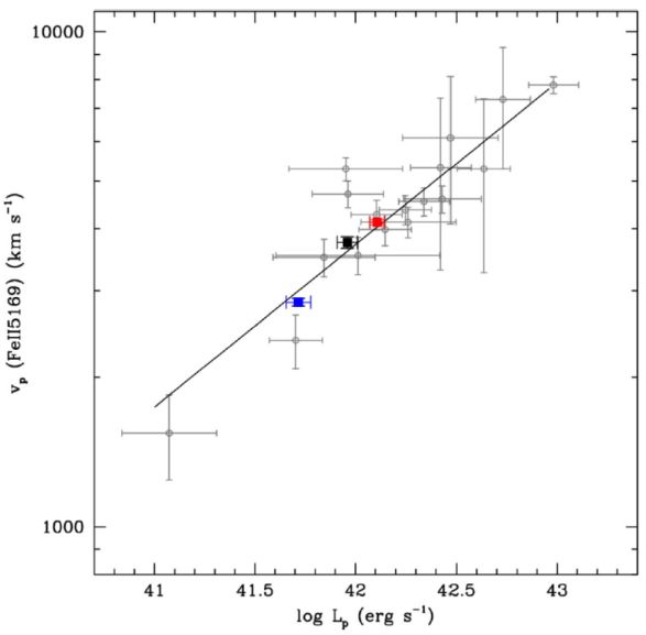 |
Figure 6. Original HP02 plane, with the positions of the homogeneously studied SNe 2012A (blue), 2012aw (red) and 2012ec (black). Plot from Barbarino et al (2015), reproduced by kind permission. |
At the present time, we still lack a homogeneous and sound calibration of the SCM based only on the primary distance indicators and, on the other side, we have only a few numbers of host galaxies where type IIP SNe have been exploded and also we detected Cepheids and/or the TRGB. A first step toward this direction was provided by Hamuy (2004) and by Jang and Lee (2014), where they adopted the calibrations of the SCM published by HP02 and Olivares et al (2010), respectively, with the distances provided by Cepheids and TRGB, to estimate the Hubble constant. More recently, Polshaw et al (2015) applied the SCM to SN 2014bc, exploded in the anchor galaxy NGC 4258, for which a geometric maser distance (with an uncertainty of only 3 %, Humphreys et al 2013a) and a Cepheids distance (Fiorentino et al, 2013) is available. They applied almost all the currently available calibrations of the SCM to SN 2014bc, and compared the estimated distances with both the maser and the Cepheids distances. They found some discrepancies between the SCM-based distance moduli and the maser distance modulus, ranging from −0.38 mag to 0.31 mag. To further investigate the scatter among the available calibrations, they applied the SCM to a set of 6 type IIP SNe occurred in galaxies for which Cepheid distances were available. They obtained a Hubble diagram in the I-band with a small scatter (σI ∼ 0.16 mag), and the following SCM calibration:
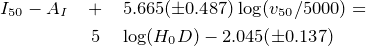 |
(1) |
where H0 = 73.8 km s−1 Mpc−1 (Riess et al, 2011), and D is the distance.
This calibration relies on the cosmic distance ladder, even if based on only a few objects. However, the derived SCM is based on Cepheid distances based on different calibrations of the Cepheid period-luminosity relations. The differences among the various calibrations are typically of the order of 0.1 mag (e.g. Fiorentino et al, 2013 and references therein). Moreover, also the adopted reddenings came from different sources, even from different calibrations of the same NaI D feature. To this aspect, we point out that current calibrations of the NaI D feature in the same galaxy may provide differences up to ∆E(B − V) ∼ 0.15 mag (see the discussion in Dall'Ora et al, 2014).
A further development of a calibration of the SCM based on primary distance indicators (Cepheids, TRGB) is highly desirable, with a larger number of calibrators and with a homogeneous analysis (i.e. same estimate of the reddening and same Cepheids period-luminosity relations and TRGB calibrations). Moreover, since the SNe calibrated on primary distance indicators occur in the local Universe, they are likely to be deeply investigated. Moreover, the progenitor could be detectable on archive images. This would allow us to fully explore the space of the structural parameters that could affect the SCM. Indeed, very recently SN LSQ13fn (Polshaw et al, 2016) was found to break the standardized candle relation. A possible explanation for that could be the low metallicity of the progenitor ( ∼ 0.1 Z⊙, Polshaw et al, 2016). As a matter of fact, theoretical models (Kasen and Woosley 2009) predict a metallicity dependence, but at the 0.1 mag level, not as large as observed in the case of SN LSQ13fn (almost 2 mag). However, a possible explanation could be a combined effect of low-metallicity of the ejecta and a strong circumstellar interactions. Whatever the case, detailed studies of nearby type IIP SNe, spanning a range of masses, metallicities and environments are of extreme importance to fully characterize the SCM.
As a final point we note that future facilities, such as E-ELT and NGST, will allow us to extend the range of the cosmological type IIP SNe, on which SCM could be applied, but also the range of local SNe, to calibrate the SCM. However, these forthcoming facilities will operate at the NIR wavelengths, therefore making it essential a sound NIR calibration of the SCM.