4.3. Measuring _m, , and q₀

In order to determine the other cosmological parameters from the supernova data we must consider supernova at large distances (z 0.3). Just as large distance measurements on Earth show us the curvature (geometry) of Earth's surface, so do large distance measurements in cosmology show us the geometry of the universe. Since, as we have seen, the geometry of the universe depends on the values of the cosmological parameters, measurements of the luminosity distance for distant supernova can be used to extract these values.

To obtain the general expression for the luminosity distance, consider photons from a distance source moving radially toward us. Since we are considering photons, ds² = 0, and since they are moving radially, d² = d² = 0. The Robertson-Walker metric, Eq. (1), then reduces to 0 = c² dt² - a² dr²(1 - k r²)^-1, which implies

(31)

To get another expression for dt, we multiply Eq. (17) by a(t)² which produces an expression for (da / dt)². Furthermore, we note that since the universe is expanding, the matter density is a function of time. Given that lengths scale as a(t), volumes scale as a(t)³ and therefore,

(32)

Using these facts, together with the definitions of the density parameters in Eq. (22), Eq. (17) becomes

(33)

As previously mentioned, it is better to write things in terms of measurable quantities, and in this case we can directly relate the cosmic scale factor to the redshift z. The redshift is defined such that

(34)

where ₀ is the current (received) value of the wavelength and is the wavelength at the time of emission. The redshift is a direct result of the cosmic expansion and it can be shown that [14] a(t) ; therefore,

(35)

Using Eq. (35) and the fact that _k = 1 - _m - from Eq. (21), Eq. (33) can be rewritten as

(36)

Equating the expressions in Eqs. (31) and (36) and integrating, leads to an expression for the radial coordinate r of the star. The luminosity distance is then given by [15] d = (1 + z) a₀r . Therefore,

(37)

where sinn(x) is sinh(x) for k < 0, sin(x) for k > 0, and if k = 0 neither sinn nor |_{k, 0}| appear in the expression. We see that the functional dependence of the luminosity distance is d (z; _m, ).

Inserting Eq. (37) into Eq. (24), and using the intercept from Eq. (28), we get a redshift-magnitude relation valid at high z

(38)

In practice, astronomers observe the apparent magnitude and redshift of a distant supernova. The density parameters are then determined by those values that produce the best fit to the observed data according to Eq. (38) for different cosmological models.

Under the continued assumption that the fluid pressure of the matter in the universe is negligible (p_m 0), Eq. (16) implies that the deceleration parameter at the present time is given by

(39)

Therefore, once the density parameters have been determined by the above procedure, the deceleration parameter can then be found.

Figure 2 illustrates how high-redshift data can be used to estimate the cosmological parameters and provide evidence in favor of a nonzero cosmological constant. In this figure, the abscissa is the difference between the distance moduli for the observed supernovae and what would be expected for a traditional cosmological model such as those represented in Table 1. The case shown is based on the data of Riess et. al. [16] using a traditional model with _m = 0.2 and = 0 represented by the central line (m - M) = 0. The figure shows that the data points lie predominantly above the zero line. This result means that the supernovae are further away (or equivalently, dimmer) than traditional, decelerating cosmological models allow. The conclusion then is that the universe must be accelerating. As suggested by Eq. (39), the most straightforward explanation of this conclusion is the presence of a nonzero, positive cosmological constant. The solid curve, above the zero line in Fig. 2, represents a best-fit curve to the data that corresponds to a universe with _m = 0.24 and = 0.72.

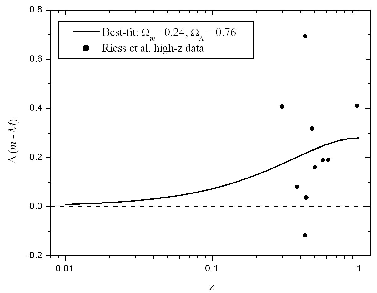Figure 2. Using high-redshift data to determine cosmological parameters and provide evidence for a nonzero cosmological constant. The zero line corresponds to a traditional decelerating model of the universe with m = 0.2, = 0, and k = 0.8. The data points are the high-redshift supernovae from Ref. 16. The solid curve corresponds to those cosmological parameters that produce a best fit to the data points as determined in Ref. 16.

Typical values for the cosmological parameters as determined by detailed analysis of the type just discussed are the following: [16]

(40)

Note that the negative deceleration parameter is consistent with an accelerating universe. Furthermore, these values imply that the universe is effectively flat predicting a curvature parameter roughly centered around _k 0.04.