6. ABSORPTION PROCESSES

6.1. Continuum versus line absorption

X-rays emitted by cosmic sources do not travel unattenuated to a distant observer. This is because intervening matter in the line of sight absorbs a part of the X-rays. With low-resolution instruments, absorption can be studied only through the measurement of broad-band flux depressions caused by continuum absorption. However, at high spectral resolution also absorption lines can be studied, and in fact absorption lines offer more sensitive tools to detect weak intervening absorption systems. We illustrate this in Fig. 9. At an O VIII column density of 10²¹ m^-2, the absorption edge has an optical depth of 1%; for the same column density, the core of the Ly line is already saturated and even for 100 times lower column density, the line core still has an optical depth of 5%.

Figure 9. Continuum (left) and Ly (right) absorption spectrum for a layer consisting of O VIII ions with column densities as indicated.

6.2. Continuum absorption

Continuum absorption can be calculated simply from the photoionisation cross sections, that we discussed already in Sect. 3.2.2. The total continuum opacity _cont can be written as

(41)

i.e, by averaging over the various ions i with column density N_i. Accordingly, the continuum transmission T(E) of such a clump of matter can be written as T(E) = exp(-_cont(E)). For a worked out example see also Sect. 6.6.

6.3. Line absorption

When light from a background source shines through a clump of matter, a part of the radiation can be absorbed. We discussed already the continuum absorption. The transmission in a spectral line at wavelength is given by

(42)

with

(43)

where ( ) is the line profile and ₀ is the opacity at the line centre ₀, given by:

(44)

Apart from the fine structure constant and Planck's constant h, the optical depth also depends on the properties of the absorber, namely the ionic column density N_i and the velocity dispersion _v. Furthermore, it depends on the oscillator strength f which is a dimensionless quantity that is different for each transition and is of order unity for the strongest transitions.

In the simplest approximation, a Gaussian profile () = exp -( - ₀)² / b²) can be adopted, corresponding to pure Doppler broadening for a thermal plasma. Here b = 2^1/2 with the normal Gaussian root-mean-square width. The full width at half maximum of this profile is given by (ln 256)^1/2 or approximately 2.35. One may even include a turbulent velocity _t into the velocity width _v, such that

(45)

with m_i the mass of the ion (we have tacitly changed here from wavelength to velocity units through the scaling / ₀ = v / c).

The equivalent width W of the line is calculated from

(46)

For the simple case that ₀ << 1, the integral can be evaluated as

(47)

A Gaussian line profile is only a good approximation when the Doppler width of the line is larger than the natural width of the line. The natural line profile for an absorption line is a Lorentz profile () = 1 / (1 + x²) with x = 4 / A. Here is the frequency difference - ₀ and A is the total transition probability from the upper level downwards to any level, including all radiative and Auger decay channels.

Convolving the intrinsic Lorentz profile with the Gaussian Doppler profile due to the thermal or turbulent motion of the plasma, gives the well-known Voigt line profile

(48)

where

(49)

and y = c / b. The dimensionless parameter a (not to be confused with the a in Eqn. 4) represents the relative importance of the Lorentzian term (~ A) to the Gaussian term (~ b). It should be noted here that formally for a > 0 the parameter ₀ defined by (44) is not exactly the optical depth at line centre, but as long as a << 1 it is a fair approximation. For a >> 1 it can be shown that H(a, 0) 1 / a^1/2.

6.4. Some important X-ray absorption lines

There are several types of absorption lines. The most well-known are the normal strong resonance lines, which involve electrons from the outermost atomic shells. Examples are the 1s-2p line of O VII at 21.60 Å, the O VIII Ly doublet at 18.97 Å and the well known 2s-2p doublet of O VI at 1032 and 1038 Å. See Richter et al. 2008 - Chapter 3, this volume, for an extensive discussion on these absorption lines in the WHIM.

The other class are the inner-shell absorption lines. In this case the excited atom is often in an unstable state, with a large probability for the Auger process (Sect. 3.2.4). As a result, the parameter a entering the Voigt profile (Eqn. 49) is large and therefore the lines can have strong damping wings.

In some cases the lines are isolated and well resolved, like the O VII and O VIII 1s-2p lines mentioned above. However, in other cases the lines may be strongly blended, like for the higher principal quantum number transitions of any ion in case of high column densities. Another important group of strongly blended lines are the inner-shell transitions of heavier elements like iron. They form so-called unresolved transition arrays (UTAs); the individual lines are no longer recognisable. The first detection of these UTAs in astrophysical sources was in a quasar (Sako et al., 2001).

In Table 6 we list the 70 most important X-ray absorption lines for < 100 Å. The importance was determined by calculating the maximum ratio W / that these lines reach for any given temperature.

Table 6. The most important X-ray absorption lines with < 100 Å. Calculations are done for a plasma in CIE with proto-solar abundances (Lodders, 2003) and only thermal broadening. The calculations are done for a hydrogen column density of 10²⁴ m^-2, and we list equivalent widths for the temperature T_max (in K) where it reaches a maximum. Equivalent widths are calculated for the listed line only, not taking into account blending by other lines. For saturated, overlapping lines, like the O VIII Ly doublet near 18.97 Å, the combined equivalent width can be smaller than the sum of the individual equivalent widths.

	ion	Wmax	log			ion	Wmax	log
(Å)		(mÅ)	Tmax		(Å)		(mÅ)	Tmax
9.169	Mg XI	1.7	6.52		31.287	N I	5.5	4.04
13.447	Ne IX	4.6	6.38		33.426	C V	7.0	5.76
13.814	Ne VII	2.2	5.72		33.734	C VI	12.9	6.05
15.014	Fe XVII	5.4	6.67		33.740	C VI	10.3	6.03
15.265	Fe XVII	2.2	6.63		34.973	C V	10.3	5.82
15.316	Fe XV	2.3	6.32		39.240	S XI	6.5	6.25
16.006	O VIII	2.6	6.37		40.268	C V	17.0	5.89
16.510	Fe IX	5.6	5.81		40.940	C IV	7.2	5.02
16.773	Fe IX	3.0	5.81		41.420	C IV	14.9	5.03
17.396	O VII	2.8	6.06		42.543	S X	6.3	6.14
17.768	O VII	4.4	6.11		50.524	Si X	11.0	6.14
18.629	O VII	6.9	6.19		51.807	S VII	7.6	5.68
18.967	O VIII	8.7	6.41		55.305	Si IX	14.0	6.06
18.973	O VIII	6.5	6.39		60.161	S VII	12.2	5.71
19.924	O V	3.2	5.41		61.019	Si VIII	11.9	5.92
21.602	O VII	12.1	6.27		61.070	Si VIII	13.2	5.93
22.006	O VI	5.1	5.48		62.751	Mg IX	11.1	5.99
22.008	O VI	4.1	5.48		68.148	Si VII	10.1	5.78
22.370	O V	5.4	5.41		69.664	Si VII	10.9	5.78
22.571	O IV	3.6	5.22		70.027	Si VII	11.3	5.78
22.739	O IV	5.1	5.24		73.123	Si VII	10.7	5.78
22.741	O IV	7.2	5.23		74.858	Mg VIII	17.1	5.93
22.777	O IV	13.8	5.22		80.449	Si VI	13.0	5.62
22.978	O III	9.4	4.95		80.577	Si VI	12.7	5.61
23.049	O III	7.1	4.96		82.430	Fe IX	14.0	5.91
23.109	O III	15.1	4.95		83.128	Si VI	14.2	5.63
23.350	O II	7.5	4.48		83.511	Mg VII	14.2	5.82
23.351	O II	12.6	4.48		83.910	Mg VII	19.8	5.85
23.352	O II	16.5	4.48		88.079	Ne VIII	15.2	5.80
23.510	O I	7.2	4.00		95.385	Mg VI	15.5	5.67
23.511	O I	15.0	4.00		95.421	Mg VI	18.7	5.69
24.779	N VII	4.6	6.20		95.483	Mg VI	20.5	5.70
24.900	N VI	4.0	5.90		96.440	Si V	16.8	5.33
28.465	C VI	4.6	6.01		97.495	Ne VII	22.8	5.74
28.787	N VI	9.8	6.01		98.131	Ne VI	16.7	5.65

Note the dominance of lines from all ionisation stages of oxygen in the 17-24 Å band. Furthermore, the Fe IX and Fe XVII lines are the strongest iron features. These lines are weaker than the oxygen lines because of the lower abundance of iron; they are stronger than their neighbouring iron ions because of somewhat higher oscillator strengths and a relatively higher ion fraction (cf. Fig. 7).

Note that the strength of these lines can depend on several other parameters, like turbulent broadening, deviations from CIE, saturation for higher column densities, etc., so some care should be taken when the strongest line for other physical conditions are sought.

6.5. Curve of growth

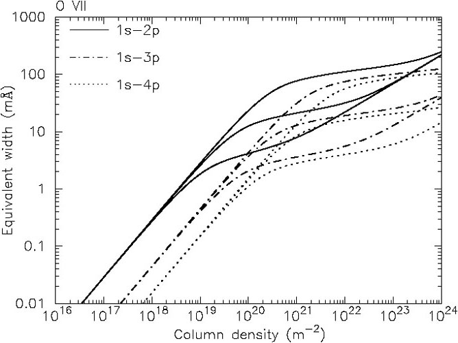
In most practical situations, X-ray absorption lines are unresolved or poorly resolved. As a consequence, the physical information about the source can only be retrieved from basic parameters such as the line centroid (for Doppler shifts) and equivalent width W (as a measure of the line strength).

As outlined in Sect. 6.3, the equivalent width W of a spectral line from an ion i depends, apart from atomic parameters, only on the column density N_i and the velocity broadening _v. A useful diagram is the so-called curve of growth. Here we present it in the form of a curve giving W versus N_i for a fixed value of _v.

The curve of growth has three regimes. For low column densities, the optical depth at line centre ₀ is small, and W increases linearly with N_i, independent of _v (Eqn. 47). For increasing column density, ₀ starts to exceed unity and then W increases only logarithmically with N_i. Where this happens exactly, depends on _v. In this intermediate logarithmic branch W depends both on _v and N_i, and hence by comparing the measured W with other lines from the same ion, both parameters can be estimated. At even higher column densities, the effective opacity increases faster (proportional to (N_i)^1/2), because of the Lorentzian line wings. Where this happens depends on the Voigt parameter a (Eqn. 49). In this range of densities, W does not depend any more on _v.

In Fig. 10 we show a few characteristic examples. The examples of O I and O VI illustrate the higher W for UV lines as compared to X-ray lines (cf. Eqn. 47) as well as the fact that inner shell transitions (in this case the X-ray lines) have larger a-values and hence reach sooner the square root branch. The example of O VII shows how different lines from the same ion have different equivalent width ratios depending on _v, hence offer an opportunity to determine that parameter. The last frame shows the (non)similarties for similar transitions in different ions. The innershell nature of the transition in O VI yields a higher a value and hence an earlier onset of the square root branch.

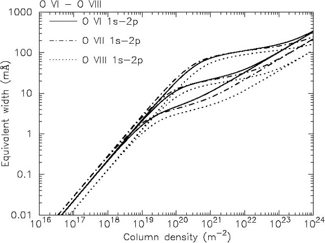Figure 10. Equivalent width versus column density for a few selected oxygen absorption lines. The curves have been calculated for Gaussian velocity dispersions = b / 21/2 of 10, 50 and 250 km s-1, from bottom to top for each line. Different spectral lines are indicated with different line styles.

6.6. Galactic foreground absorption

All radiation from X-ray sources external to our own Galaxy has to pass through the interstellar medium of our Galaxy, and the intensity is reduced by a factor of e ^{- (E)} with the optical depth (E) = _{i i}(E) n_i() d, with the summation over all relevant ions i and the integration over the line of sight d. The absorption cross section _i(E) is often taken to be simply the (continuum) photoionisation cross section, but for high-resolution spectra it is necessary to include also the line opacity, and for very large column densities also other processes such as Compton ionisation or Thomson scattering.

For a cool, neutral plasma with cosmic abundances one often writes

(50)

where the hydrogen column density N_H n_H dx. In _eff(E) all contributions to the absorption from all elements as well as their abundances are taken into account.

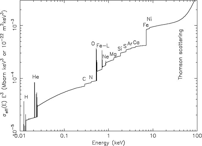
The relative contribution of the elements is also made clear in Fig. 11. Below 0.28 keV (the carbon edge) hydrogen and helium dominate, while above 0.5 keV in particular oxygen is important. At the highest energies, above 7.1 keV, iron is the main opacity source.

Figure 11. Left panel: Neutral interstellar absorption cross section per hydrogen atom, scaled with E3. The most important edges with associated absorption lines are indicated, as well as the onset of Thompson scattering around 30 keV. Right panel: Contribution of the various elements to the total absorption cross section as a function of energy, for solar abundances.

Yet another way to represent these data is to plot the column density or distance for which the optical depth becomes unity (Fig. 12). This figure shows that in particular at the lowest energies X-rays are most strongly absorbed. The visibility in that region is thus very limited. Below 0.2 keV it is extremely hard to look outside our Milky Way.

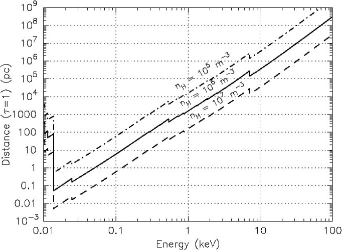Figure 12. Left panel: Column density for which the optical depth becomes unity. Right panel: Distance for which = 1 for three characteristic densities.

The ISM contains cold gas (< 50 K), warm, neutral or lowly ionised gas (6000 - 10000 K) as well as hotter gas (a few million K). We have seen before (see Sect. 3.2.2) that for ions the absorption edges shift to higher energies for higher ionisation. Thus, with instruments of sufficient spectral resolution, the degree of ionisation of the ISM can be deduced from the relative intensities of the absorption edges. Cases with such high column densities are rare, however (and only occur in some AGN outflows), and for the bulk of the ISM the column density of the ionised ISM is low enough that only the narrow absorption lines are visible (see Fig. 9). These lines are only visible when high spectral resolution is used (see Fig. 13). It is important to recognise these lines, as they should not be confused with absorption line from within the source itself. Fortunately, with high spectral resolution the cosmologically redshifted absorption lines from the X-ray source are separated well from the foreground hot ISM absorption lines. Only for lines from the Local Group this is not possible, and the situation is here complicated as the expected temperature range for the diffuse gas within the Local Group is similar to the temperature of the hot ISM.

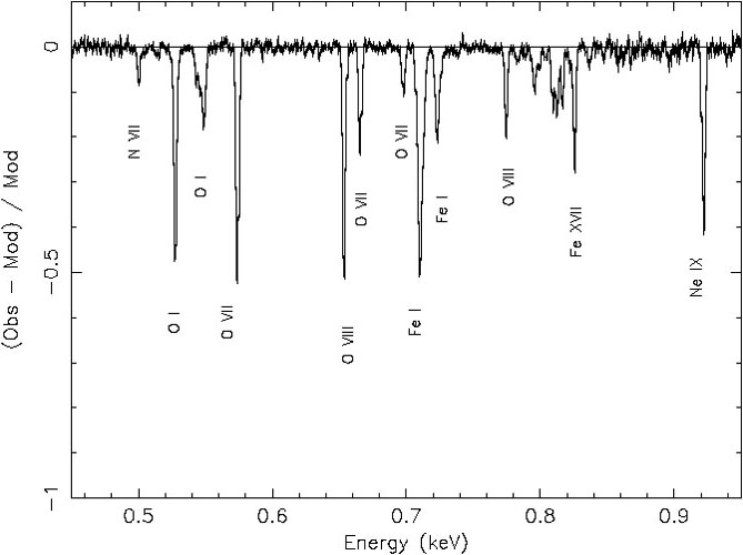
Figure 13. Left panel: Simulated 100 ks absorption spectrum as observed with the Explorer of Diffuse Emission and Gamma-ray Burst Explosions (EDGE), a mission proposed for ESA's Cosmic Vision program. The parameters of the simulated source are similar to those of 4U 1820-303 (Yao & Wang, 2006). The plot shows the residuals of the simulated spectrum if the absorption lines in the model are ignored. Several characteristic absorption features of both neutral and ionised gas are indicated. Right panel: Simulated spectrum for the X-ray binary 4U 1820-303 for 100 ks with the WFS instrument of EDGE. The simulation was done for all absorbing oxygen in its pure atomic state, the models plotted with different line styles show cases where half of the oxygen is bound in CO, water ice or olivine. Note the effective shift of the absorption edge and the different fine structure near the edge. All of this is well resolved by EDGE, allowing a determination of the molecular composition of dust in the line of sight towards this source. The absorption line at 0.574 is due to highly ionised O VII.

Another ISM component is dust. A significant fraction of some atoms can be bound in dust grains with varying sizes, as shown below (from Wilms et al. 2000):

The numbers represent the fraction of the atoms that are bound in dust grains. Noble gases like Ne and Ar are chemically inert hence are generally not bound in dust grains, but other elements like Ca exist predominantly in dust grains. Dust has significantly different X-ray properties compared to gas or hot plasma. First, due to the chemical binding, energy levels are broadened significantly or even absent. For example, for oxygen in most bound forms (like H₂O) the remaining two vacancies in the 2p shell are effectively filled by the two electrons from the other bound atom(s) in the molecule. Therefore, the strong 1s-2p absorption line at 23.51 Å (527 eV) is not allowed when the oxygen is bound in dust or molecules, because there is no vacancy in the 2p shell. Transitions to higher shells such as the 3p shell are possible, however, but these are blurred significantly and often shifted due to the interactions in the molecule. Each constituent has its own fine structure near the K-edge (Fig. 13b). This fine structure offers therefore the opportunity to study the (true) chemical composition of the dust, but it should be said that the details of the edges in different important compounds are not always (accurately) known, and can differ depending on the state: for example water, crystalline and amorphous ice all have different characteristics. On the other hand, the large scale edge structure, in particular when observed at low spectral resolution, is not so much affected. For sufficiently high column densities of dust, self-shielding within the grains should be taken into account, and this reduces the average opacity per atom.

Finally, we mention here that dust also causes scattering of X-rays. This is in particular important for higher column densities. For example, for the Crab nebula (N_H = 3.2 × 10²⁵ m^-2), at an energy of 1 keV about 10% of all photons are scattered in a halo, of which the widest tails have been observed out to a radius of at least half a degree; the scattered fraction increases with increasing wavelength.