


As we go from gas-rich spiral systems to early-type galaxies (ETGs) or dwarf spheroidals (dSphs), common practice is to abandon the systematic use of the extended neutral gas component of the former as a tracer to determine the mass distribution. However, many ETGs have a significant amount of gas, either ionised (e.g. Bertola et al. 1984; Fisher 1997; Sarzi et al. 2006), sometimes molecular (e.g. Sage et al. 2007; Young et al. 2011) or even neutral (Knapp et al. 1985; Morganti et al. 2006; di Serego Alighieri et al. 2007). In such cases, it is possible to conduct parallel approaches to constrain the overall mass profiles of the galaxies. This has been exploited in the context of, say, the search for supermassive black holes (see e.g. Neumayer 2010), the kinematics of the central regions (Corsini et al. 1999; Vega Beltrán et al. 2001; Pizzella et al. 2004; Sarzi et al. 2006, and references therein) or large-scale kinematics (Franx et al. 1994; Weijmans et al. 2008).
However, the scarcity and complexity of observed gaseous distributions and kinematics and the associated difficulty of properly modelling the dissipative content of galaxies with multi-component morphologies though (see e.g. Weiner et al. 2001) has led to further reliance on stellar dynamics: the interpretation of the large- (and small-) scale rotation curves revealed by the emitting gaseous content has thus generally been overtaken by state-of-the-art modelling of one of the existing dissipationless tracer, e.g. old stars, globular clusters, planetary nebulae. The associated side-products, i.e., constraints on the orbital structure of the galaxy under scrutiny, have the advantage of representing a rich source of information to establish its overall formation and evolution history.
In the following sub-sections, we will therefore restrict ourselves to briefly introducing the basic ingredients needed for the kinematic modelling of dissipationless systems, i.e., the determination of the total mass distribution, thus yielding the dark matter (DM) distribution after subtraction of the visible component. Determining the mass distribution requires extending beyond the simple use of the first velocity moment, the mean velocity V, as the centered second velocity moment, the stellar velocity dispersion σ, becomes a non-negligible actor. Orbital shapes also depart from the commonly-assumed circularity. Kinematic modelling is significantly more accurate through the measurement of the detailed shape of the velocity distribution, which is directly related to the orbital shapes, and thus allowing a better understanding of the formation of the galaxies under study.
We first provide some insights on the dependence of mass estimators based on the measurement of the line-of-sight (LOS) velocity dispersion on details of the probed aperture. We then describe the standard techniques of kinematic modelling, based upon either the Jeans equations of local dynamical equilibrium or the six-dimensional distribution functions and we highlight the recent improvements to these methods. We finally illustrate the power of these methods with recent analyses of observed gas-poor galaxies, often obtaining useful constraints on the compatibility of the DM profiles with those in ΛCDM halos. In several cases, one can also obtain useful constraints on the DM normalization, concentration, inner slope, as well as the orbital velocity anisotropy (hereafter anisotropy) in the inner and outer regions. This review does not specifically address the mass modelling of central supermassive black holes (see references in, e.g. Kormendy & Ho 2013), however most of the techniques that we discuss here also apply to that problem. The reader is also referred to Gerhard (2013) for another recent review on dark matter profiles determinations based on multiple tracers.
Before engaging in the complexity of the mass modelling described in Section 5.3, we review simple mass estimators that have been proposed, all based on the scalar virial theorem (sVT).
The sVT states that for an isolated system in steady state
 |
(24) |
where the total kinetic energy K = 1/2 M ⟨v2⟩, M is the total galaxy mass and ⟨v2⟩ is the mean square velocity of its stars, integrated over the entire galaxy, while W is the total potential energy, which depends on the distribution of the stars and the possible dark matter. This energy budget derives from a time average and depends on the isolation of the dynamical system (to ensure that the tracer is not affected by a neighboring system).
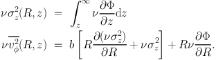
For a non-rotating spherical galaxy, the mean square velocity of the stars is related to the observed LOS velocity dispersion: ⟨v2 ⟩ = 3⟨ σlos2⟩ (where both averages extend to infinity). Assuming finite mass, Eq. (24) gives
 |
(25) |
where rr is a characteristic radius of the galaxy, while c = 6 M2 / {rr ∫0∞[M(r) / r]2 dr}, in the self-consistent case. When the ⟨σlos2⟩ integral is extended over the entire galaxy, Eq. (25) is completely independent on the radial variation of the stellar anisotropy (Binney & Tremaine 2008, Section 4.8.3). In the general case, the coefficient c depends uniquely on the total (ρ) and tracer (ν, i.e. stellar in galaxies) density profiles of the system.
The practical application of that formula has been the source of some confusion to be addressed before engaging into tentative interpretations. Firstly, the physical radius rr is measured by the angular radius that it subtends; therefore, it depends directly on the assumed distance D of the object. Any uncertainty on D thus translates linearly into M. Secondly, there is an inherent uncertainty associated with rr's measurement: while it can be strictly defined as, for example, the radius at which half of the galaxy's total light is encompassed, the notion of total light itself is ill-defined (it often depends on a subjective extrapolation); the nature of the data also plays a role (e.g. bandpass and signal-to-noise effects). It is thus common to retrieve specific radii values differing by factors of two or more for the same well-studied systems (e.g. Kormendy et al. 2009; Chen et al. 2010). Both issues should be carefully addressed, especially when considering samples of galaxies for which distances and aperture radii emerge from heterogeneous sources and/or methods. Thirdly, when working at a finite radius rr, one must add a non-negligible surface term into the virial theorem (The & White 1986).
The application of Eq. (25) as a robust mass estimator is further compounded by its limited applicability to real stellar systems: one can rarely observe the stellar σlos for the entire galaxy, due to the rapid surface brightness drop with galactocentric radii. Therefore, the effect of using a finite aperture must be considered (Michard 1980; Bailey & MacDonald 1981; Tonry 1983). In early works, the coefficient c was only determined for specific galaxy surface brightness profiles (Poveda 1958; Spitzer 1969). Using Jeans models, it was realized that the coefficient c however depends significantly on the shape of galaxy surface brightness profile and on the dynamical structure of the galaxy (that is, its anisotropy, see e.g. Prugniel & Simien 1997; Bertin et al. 2002).
Moreover, galaxies contain unknown amounts of dark matter, making the total mass M an uncertain and ill-defined quantity. For these reasons, following Trujillo et al. (2004), we rewrite Eq. (25) as
 |
(26) |
where the σlos and mass integrals are restricted to finite radii, and where
 |
(27) |
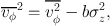
is the squared aperture velocity dispersion averaged over a cylindrical aperture on the sky of projected radius Rσ.
Cappellari et al. (2006) calibrated Eq. (26) using the observed surface distributions and integral-field kinematics within typically the effective radius containing half the projected luminosity, Re, for a sample of ETGs, in combination with Schwarzschild's axisymmetric dynamical models. They found that the enclosed mass within the effective radius (rr = Re) of ETGs can be robustly recovered using a best-fitting coefficient 8 c ≈ 2.5, which varies little from galaxy to galaxy, with rM = r1/2light (the radius of a sphere enclosing half of the galaxy light) and with rr = Rσ = Re (the radius of a cylinder enclosing half of the galaxy light). Using rM = r1/2light, rr = Re and Rσ → ∞, Wolf et al. (2010) analytically derived c ≃ 4.0 for systems with σlos(R) ≈ Cst and proved that c depends very little on anisotropy (as expected given their infinite aperture for σap). 9
| Spitzer | Cappellari | Wolf | 3 Re | |
| rM | ∞ | r1/2light | r1/2light | 3 Re |
| rr | r1/2 | Re | Re | Re |
| Rσ | ∞ | Re | rvir | 3 Re |
| Predicted | 7.5 | 2.5 | 4.0 | — |
| Hernquist | 7.46 | 3.31 | 4.84 | 5.74 |
| n=2.0 Sérsic | 7.23 | 3.63 | 4.85 | 7.22 |
| n=4.0 Sérsic | 6.59 | 2.96 | 4.44 | 5.36 |
| n=5.5 Sérsic | 5.91 | 2.49 | 3.96 | 4.37 |
| n=2.0 Sérsic + Einasto DM | 112 | 3.74 | 4.96 | 8.38 |
| n=4.0 Sérsic + Einasto DM | 103 | 3.20 | 4.33 | 6.70 |
| n=5.5 Sérsic + Einasto DM | 94 | 2.76 | 3.95 | 5.70 |
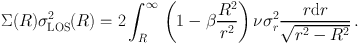
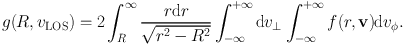
Table 2 lists the values of c for some popular models of elliptical galaxies for comparison with different predictions (assuming isotropic velocities; anisotropic velocities are discussed later). The values of c are computed by inserting the LOS velocity dispersion of Eq. (34) into Eq. (27), yielding
 |
(28) |
where ν(r) and Mp(R) are the stellar mass density at r and stellar mass enclosed in the cylinder of radius R, and where the denominator is obtained, for isotropic orbits, by Mamon & Łokas (2005a; 2006). 10 Note that our models are idealized as they do not include realistic kinematics, galaxy rotation or multiple photometric components as in the real stellar systems on which the estimators were originally calibrated. The first three models (from Hernquist 1990 and Sersic 1968) assume no DM, while the last three include an m = 6 Einasto DM model (which Navarro et al. 2004 first found to fit best the halos in ΛCDM pure DM simulations), with radius of density slope -2 equal to one tenth the quasi-virial radius, r200, 11 within which the DM accounts for 90% of the total.
For the Cappellari et al. and especially the Wolf et al. estimators, the mass within r1/2 depends little on the DM (the Spitzer relation, originally formulated for single-component polytropes, with rM = r1/2light, matches that of Wolf et al., except for the Hernquist model, where c = 4.96). Inclusion of velocity anisotropy, with β = r/2/(r + aβ) (Mamon & Łokas 2005b), where aβ = 2 Re as found for ellipticals formed by mergers by Dekel et al. (2005), makes no difference when Rσ → ∞ (as theoretically expected) and decreases c by typically only 4% for finite Rσ.
In general, galaxies are not spherical and rotate. For this reason, Eq. (26) is not rigorously correct. However, for an aperture that extends to 1Re, Eq. (26) was empirically found to still provide a reliable enclosed-mass estimator (Cappellari et al. 2006; 2013b). In this case, σe is measured from a single 'effective' spectrum within an aperture, centered on the galaxy, enclosing half of the galaxy light. The spectrum can be obtained from integral-field observations for nearby galaxies, or from a single aperture for high-redshift ones. The resulting σe2 provides a good approximation to the luminosity-weighted velocity second moment v2LOS ≈ V2 + σ2 inside the given aperture, where V is the observed mean stellar velocity at a given location and σ is the corresponding dispersion. For this reason, σe automatically includes contributions from both rotation and velocity dispersion and is only improperly called σ. The inclusion of rotation is essential for the reliability of the mass estimator.
The Spitzer (1969) and Wolf et al. (2010) formulae require kinematic measurements out to the virial radius 12. Such data can currently be obtained only for dSph's or globular clusters using individual stellar velocities. When those data are available, the latter formula is weakly sensitive to the differences in the input models. However, the Cappellari et al. (2006) formula should be used instead when only central kinematics (within ~ 1 Re) is available, as is currently the case for most ETGs. The data in Table 2 suggest that most of the difference in the coefficients c of Cappellari et al. and Wolf et al. is attributable to their use of different apertures to measure kinematics. Incidentally, both formulae provide formally correct results for a self-consistent Sérsic model with m = 5.5, where the difference in c is entirely explained by the different apertures.
Table 2 also illustrates that aperture averaged velocity dispersions out to 3 Re are insufficient to measure the DM fraction at that radius (which is determined more accurately using the radial profile σlos(R) out to 3 Re).
Below, we consider the more refined methods for determining the distribution of total mass of ETGs lacking a spatially extended gas tracer.
5.3. Methods based on Dynamical Modelling
The mass distribution in a gas-poor (and luminous) galaxy is expected to be generally dominated by baryons (mostly stars) in the inner parts and DM-dominated in the outskirts. The exact location and shape of the transition between these two regimes has been the subject of an active debate, with conclusions that seem to depend on the type (and mass) of the sampled galaxies.
The density profiles of DM halos in dissipationless ΛCDM simulations (hereafter ΛCDM halos) seem to converge (Navarro et al. 2004) to the "Einasto" model (e.g. Einasto & Haud 1989), which is mathematically "prettier" than the traditional Navarro et al. (1996b, hereafter NFW) model as its central density and total mass are both, unlike NFW, finite. These fits are now established from ≃ 10-3 (Navarro et al. 2010) to 2 or 3 (Prada et al. 2006) virial radii.
The inclusion of dissipative gas in cosmological simulations has the effect of concentrating the baryons in the centers of their structures, where they dominate the gravitational potential and drive the DM component deeper inside. On the scales of ETGs, this effect, commonly referred to as adiabatic contraction (Blumenthal et al. 1986; Gnedin et al. 2004) alters the DM density profile towards the singular isothermal (ρ ∝ 1/r2) model. This result is, however, expected to be very sensitive to the details of the baryonic feedback processes, and orbit diffusion by the quickly varying potential could be an important agent in flattening of the DM halo cusp (e.g. Pontzen & Governato 2012). See more discussion on this issue in Section 3.3.1.
For all galaxy types, the dissipative nature of baryons leads them to accumulate in galaxy centers; indeed, if the baryons were negligible everywhere, the Einasto (or NFW) models found in ΛCDM halos would lead to much lower local stellar M / L and aperture velocity dispersion than observed (Mamon & Łokas 2005a). The dominance of baryons in the center and of DM in the envelopes of ETGs has been confirmed by X-ray measurements (Humphrey et al. 2006; Humphrey & Buote 2010) and dynamical modelling (e.g. Cappellari et al. 2006; Thomas et al. 2011b); see Section 5.5 below.
In the central region (within ~ 1-2 Re) of an ETG, we rely on a tracer that may generate the majority of the local potential, making the stars a nearly self-consistent component of the galaxy 13. This would contrast with the galaxy's outskirts, where the potential would be completely dominated by invisible matter, and our visible tracers are merely a set of orbiting entities.
The holy grail of dynamicists is the distribution function (hereafter DF), that is the density in phase space (the union of position and velocity spaces) of the observed tracer (luminosity for unresolved ETGs, numbers of stars for resolved dSphs). Its evolution is set by the collisionless Boltzmann equation (hereafter CBE), which states the incompressibility of the system in 6-dimensional phase space, or in simpler terms that the DF, f, is conserved along trajectories (df / dt = 0). In vector notation, the CBE reads:
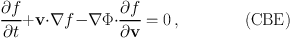 |
where Φ is the gravitational potential. In the last term, - ∇ Φ is the force per unit mass acting on stars (and other bodies). The total density ρ is uniquely determined from Φ through the Poisson equation:
 |
Solving the CBE coupled with the Poisson equation is a challenging task, especially since f is a function of at least 6 variables (3 positions, 3 velocities, ignoring any time dependence), and one can rarely access the tracers representing the total density ρ. A way out of this conundrum is to consider local variables, to eliminate the direct dependence of f with respect to velocities, as detailed below.
The traditional simpler approach to mass modeling involves writing the first velocity moments of the CBE, yielding the Jeans equations 14 that specify the local dynamical equilibrium
 |
(29) |
where ν = ∫ f d3 v is the space density of the tracer, σ2 is the tracer's dispersion tensor, whose elements are σij2 = vi vj - vi vj, where ν vi = ∫ vi f d3 v and ν vi vj = ∫ vi vj f d3 v. The product ν σ2 represents the anisotropic dynamical pressure tensor of the tracer.
The CBE and the Jeans equations (Eq. 29) apply to all systems, even out of dynamical equilibrium, as long as the tracers behave like test particles in the gravitational potential, hence do not interact (otherwise the right-hand-side of the CBE would be non-zero). In other words, the two-body relaxation time must be much longer than the age of the Universe, as is the case for ETGs, dEs (except in their nuclei) and dSphs. In particular (as mentioned above), in both the CBE and the Jeans equations, there is no requirement that the observed tracer density, ν, be proportional to the total mass density, ρ.
With the simplifying assumptions of stationarity (ignoring any direct time dependence, i.e. removing the first term on the left-hand side of the CBE), these stationary Jeans equations specify the local dynamical equilibrium:
 |
(30) |
Using the stationary Jeans equations (Eq. 30), one can relate the orbital properties, contained in the streaming (1st) and pressure (2nd) terms with the mass distribution contained in the potential (right-hand-side), through Poisson's equation. Such a Jeans analysis is fairly simple, as it circumvents the difficult problem of recovering the DF, by only considering its first few moments, which more directly relate to real astronomical observable quantities (depending on spatial coordinates). However, one is still left with a degeneracy between mass and the anisotropy of the pressure tensor, as we will discuss in the following subsections. Moreover, using moments does not guarantee that the DF is positive or null everywhere (Newton & Binney 1984).
The small departures from circular symmetry of many astrophysical systems observed in projection, such as globular clusters, dSphs and the rounder early-type galaxies as well as groups and clusters of galaxies, has encouraged dynamicists to often assume spherical symmetry in their kinematic modelling. The stationary non-streaming spherical Jeans equation can then be simply written
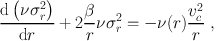 |
(31) |
where ν σr2 is the radial dynamical pressure (hereafter radial pressure), vc2(r) = GM(r) / r = r dΦ / dr is the squared circular velocity at radius r, while M(r) is the total mass profile, and where
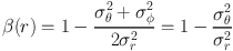 |
(32) |
is the tracer's anisotropy profile with σr ≡ σrr, etc., σθ = σφ, by spherical symmetry, and with β = 1, 0, → -∞ for radial, isotropic and circular orbits, respectively. The stationary non-streaming spherical Jeans equation provides an excellent estimate of the mass profile, given all other 3D quantities, in slowly-evolving triaxial systems such as ΛCDM halos (Tormen, Bouchet, & White 1997) and for the stars in ETGs (e.g. formed by mergers of gas-rich spirals in dissipative N-body simulations; Mamon et al. 2006).
As one is left with two unknown quantities, the radial profiles of mass and anisotropy, linked by a single equation, one must contend with a nefarious mass-anisotropy degeneracy (MAD). The simplest and most popular approach to circumvent the MAD is to assume simply parameterized forms for both the mass and anisotropy profiles. One can then express the product of the observable quantities: the surface density profile, Σ(R), and the line of sight square velocity dispersion profile, σlos2(R), versus projected radius R through the anisotropic kinematic projection equation (Binney & Mamon 1982) expressing the observed quantity
 |
(33) |
One can insert the radial pressure from the spherical stationary Jeans Eq. (31) into Eq. (33) to determine the line-of-sight (LOS) velocity dispersions through a double integration over ν M dr. Mamon & Łokas (2005b, Appendix) have simplified the problem by writing the projected pressure as a single integral
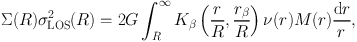 |
(34) |
where they determined simple analytical expressions for the dimensionless kernel Kβ for several popular analytical formulations of β(r; rβ) (Tremaine et al. 1994 previously derived Kβ(r, R) = √1 - R2 / r2 for β = 0). The number density ν is obtained by Abel inversion
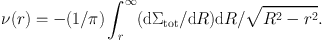 |
When both ρ(r) and ν(r) are expanded as sums of spherical Gaussian functions (Bendinelli 1991), Eq. (34) can be applied to the individual Gaussians, which can have different β values. This leads to an expression involving a single quadrature for nearly general β(r) profiles (Cappellari 2008).
The next step in complexity is the non-parametric mass inversion, where β(r) is assumed, involving first the anisotropic kinematic deprojection by inverting Eq. (33) (Mamon & Boué 2010; Wolf et al. 2010) and then directly obtaining the mass profile by inserting the derived radial pressure into the Jeans Eq. (31). For simple β(r) models, the mass profile can be written as a single integral (Mamon & Boué 2010). Interestingly, for systems with roughly constant σlos(R) (as is the case for most galaxies), the mass profile at the half-light radius r1/2 ≃ 1.3 Re is almost independent of the assumed β(r), as analytically derived by Wolf et al. (2010).
Alternatively, a mass profile is assumed and one directly determines the anisotropy profile through the non-parametric anisotropy inversion, first derived by Binney & Mamon (1982), with other algorithms by Tonry (1983), Bicknell et al. (1989), Dejonghe & Merritt (1992), and especially Solanes & Salvador-Solé (1990).
None of these approaches can lift the MAD. One promising alternative approach is to consider the variation with projected radius of the LOS velocity dispersion and kurtosis (Łokas 2002; Łokas & Mamon 2003). This method has been successfully tested (Sanchis et al. 2004) on ΛCDM halos viewed in projection, despite the fact that these halos are triaxial (Jing & Suto 2002a, and references therein), with anisotropy that increases with radius (Mamon & Łokas 2005b, and references therein), substructures and streaming motions. Unfortunately, the LOS projection of the 4th order Jeans equation, required in the dispersion-kurtosis method, is only possible when β = Cst, whereas ETGs formed by major mergers show rapidly increasing β(r) (Dekel et al. 2005). Nevertheless, Richardson & Fairbairn (2013a) recently generalized this approach for systems where the 4th order anisotropy is a function of the usual 2nd order one, as is indeed seen in ΛCDM halos (Wojtak et al. 2008).
Still, the large majority of the galaxies in the Universe are to first order axisymmetric (except for spiral arms and bars) and possess disks even for ETGs (McDonald et al. 2011; Krajnović et al. 2011). This includes fast-rotators (Emsellem et al. 2007; Cappellari et al. 2007; Emsellem et al. 2011) and spirals.
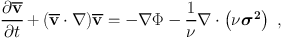
If we rewrite the stationary CBE in cylindrical coordinates (R, z, φ) and assume axial symmetry and steady state, we obtain two non-trivial Jeans equations (Jeans 1922; Binney & Tremaine 2008, Eq. 4.222b,c) that are functions of four unknowns, σR2, σz2, v2φ, and vR vz and do not uniquely specify a solution. By assuming that the velocity-ellipsoid is aligned with the cylindrical coordinates, we further simplify such equations as:
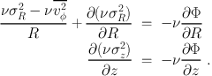 |
(35) (36) |
The two Eqs. (35) and (36) now depend only on σR2, σz2, v2φ, but one must still specify at least one function of (R, z) for a unique solution.
The generality of such equations can be maintained by writing a direct dependence between the two dispersions in the meridional plane via a function b such that σR2 = b σz2, with the boundary condition νσz2 = 0 as z → ∞. This yields (e.g. Cappellari 2008)
 |
(37) (38) |
For a given observed surface brightness and assumed total mass distribution, when Eqs. (37) and (38) are projected onto the plane of the sky and integrated along the LOS, they produce a unique prediction for the observed 2nd moment v2LOS, as a function of b and the inclination i. The 2nd moment v2LOS is empirically well approximated by vrms2 ≡ V2 + σ2 (the squares of the centroid of a Gaussian fit to the LOS velocity profile and of its dispersion), which is easily observed in galaxies. This implies that V and σ do not provide separately any extra information on the galaxy mass that is not already contained in their quadratic sum. It also implies that, when galaxy rotation V is significant, one cannot neglect its contribution to the galaxy mass determination, and that one needs to know the inclination of the galaxy accurately. The dependence of the mass distribution on Vrms alone can be physically understood: for a given dynamical model, any star along a given orbit can have its sense of rotation reversed without altering v2LOS (or the mass).
To predict galaxy rotations from the Jeans equations one must make an extra assumption on how the 2nd moments around the symmetry axis v2φ divides into ordered and random motions: v2φ = v2φ + σφ2. The simplest assumption to define this division is to adopt an oblate velocity ellipsoid (OVE), namely assume σφ = σR > σz (Cappellari 2008). This OVE model has a streaming velocity uniquely defined by
 |
(39) |
with v2φ and σz2 as given in Eqs. (37) and (38).
With b = 1, Eqs. (37) and (38) define a circular velocity-ellipsoid in the (vR, vz) plane: this is the historical semi-isotropic assumption that implies σR = σz (and vR vz = 0), and is sufficient to 'close' the set of equations to provide a unique solution for the remaining variables σz2 and v2φ (Nagai & Miyamoto 1976; Satoh 1980; Binney et al. 1990; van der Marel et al. 1990; Emsellem et al. 1994). If we consider Eq. (39), we retrieve the special case of the classic isotropic rotator (Binney 1978).
When the total mass and surface brightness are described via the Multi-Gaussian Expansion (MGE) method of Emsellem et al. (1994), the potential and Jeans Equations can be expressed in a simple form and v2LOS only requires a single quadrature both for the semi-isotropic case (Emsellem et al. 1994; 1999). This is also true for the general case σR ≠ σz ≠ σφ, and for all the six projected second moments, including radial velocities and proper motions, as demonstrated by Cappellari (2008). This flexibility can be more practically witnessed when using an implementation of the "Jeans Anisotropic MGE" (JAM) modelling method (see Cappellari 2008) augmented by the possibility to probe the parameter space within a Bayesian framework (e.g. Section 2.3.2). A key feature of the OVE rotator with constant b = (σR / σz)2 is that it maintains the simplicity of the isotropic (or semi-isotropic) rotator, but contrary to the latter, it provides a remarkably good description of the observations. In fact, these suggest that both fast-rotator ETGs (Cappellari et al. 2007; Thomas et al. 2009) and disk galaxies have a dynamical structure roughly characterized by a flattening of the velocity ellipsoid in the z direction parallel to the galaxy symmetry axis (Gerssen et al. 1997; Gerssen et al. 2000; Shapiro et al. 2003; Noordermeer et al. 2008). Indeed, once an accurate description of the surface brightness of the galaxies is provided via the MGE, the OVE rotator with constant b accurately predicts (Figure 15) both the first (V) and 2nd (Vrms = √Vrot2 + σ2) moment of the LOS velocity as inferred with state-of-the-art integral-field observations of the stellar kinematics of large samples of fast-rotator ETGs (Cappellari 2008; Scott et al. 2009; Cappellari et al. 2013b). The success of the cylindrical oriented approximation may be related to the disk-like nature of the majority of the galaxies in the Universe, where this particular alignment of the velocity ellipsoid appears natural (Richstone 1984).
 |
Figure 15. Data-model comparison of six fast rotator galaxies (previously classified as either E's and S0's) using the "Jeans Anisotropic MGE" (JAM) method from Cappellari (2008). From top to bottom: bi-symmetrized observations of Vrms ≡ √V2 + σ2, model of same, bi-symmetrized observations of V, model of V. The contours show the isophotes. The models generally agree with the original non-symmetrized data within the statistical errors. |
Real galaxies need not have accurately cylindrically oriented velocity ellipsoids. In fact, theoretical arguments and numerical experiments suggest the velocity ellipsoid cannot be perfectly cylindrically oriented (e.g. Dehnen & Gerhard 1993). However, comparison with realistic N-body simulations of galaxies indicate that the cylindrically-oriented velocity ellipsoid approximation can be used to reliably measures the mean values of the internal anisotropy or to recover mean M / L even in realistic situations where the anisotropy is not constant (Lablanche et al. 2012).
5.4. Distribution Function Analysis
Although the Jeans analysis is simple and fast, it has two disadvantages: firstly, the 2nd LOS velocity moment does not describe the full information of projected phase space (hereafter, PPS) (α,δ,vlos), where (α, δ) are the equatorial sky coordinates and vlos is the LOS velocity), and even the inclusion of the higher order moments (see e.g. Magorrian & Binney 1994; Magorrian 1995) is less informative than using the full PPS; Secondly, for spherically modeled galaxies, the solutions of the Jeans analysis depend on the required radial binning of the velocity moments. Moreover, the variation of the velocity moments with projected radius is often noisy, requiring smoothing of the data. We now describe a more general family of mass modelling methods, which solves for the gravitational potential and the DF, by fitting the PPS distribution predicted for combinations of gravitational potential and DF to the observed PPS distribution.
5.4.1. Spherical Distribution Function Modelling
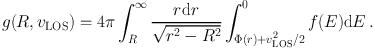
In spherical symmetry, the PPS is simply (R, vlos), where R is the projected radius, and the DF projects onto PPS as a triple integral (Dejonghe & Merritt 1992):
 |
(40) |
So, with the knowledge of the DF shape, one can fit its parameters to match the PPS.
In spherical systems with isotropic non-streaming velocities, the DF is a function of energy only, i.e. f = f(E), while in anisotropic non-streaming (e.g., non-rotating) spherical systems it is a function of energy and the modulus of the angular momentum. The PPS distribution in isotropic systems is (Strigari et al. 2010)
 |
(41) |
where the DF is given by the Eddington formula (Eddington 1916).
However, ΛCDM halos are anisotropic (e.g. Colín et al. 2000; Ascasibar & Gottlöber 2008). Wojtak et al. (2008) have recently shown that ΛCDM halos have DFs that are separable in energy and angular momentum, with f(E, L) = fe(E) L2 (β∞ - β0) (1 + L2 / L02)-β0, with β0 = β(0) and β∞ = limr→∞ β, and where L0 is a free parameter related to the "anisotropy radius" where β(r) = (β0 + β∞) / 2. Unfortunately, the energy part of the DF is non-analytical, though Wojtak et al. show how it can be efficiently evaluated numerically (they also provide an analytical approximation for fe(E)). This ΛCDM halo-based DF can then be applied to fit the distribution of objects in PPS using Eq. (40), as shown by Wojtak et al. (2009).
For quasi-spherical galaxies, where, in contrast to clusters and ΛCDM halos, dissipation ought to play an important role, it is not yet clear that the DF is separable in energy and angular momentum as Wojtak et al. (2008) have found for ΛCDM halos. Moreover, the triple integral in Eq. (40) makes the ΛCDM halo DF method computationally intensive. The simplest and popular alternative is to fit the PPS assuming a Gaussian distribution for the LOS velocities, and the radial profiles of mass and anisotropy (Battaglia et al. 2008; Strigari et al. 2008; Wolf et al. 2010). Unfortunately, this method provides very weak constraints on the anisotropy (Walker et al. 2009b). 15 One can assume instead a Gaussian shape for the 3D velocity distribution, as in the MAMPOSSt method of MBB13, again adopting radial profiles of mass and anisotropy, and fitting the predicted distribution of particles in PPS. This operation only involves a single integral.
Both the ΛCDM halo DF and MAMPOSSt methods have been successfully tested on ΛCDM halos viewed in projection (Wojtak et al. 2009; Mamon et al. 2013, respectively). They both yield useful constraints on both the mass and anisotropy profiles: with ~500 tracers, the mass M200 within the (quasi-virial) radius r200 and the outer anisotropy are recovered with ~ 30% and ~ 20% relative accuracy, while the scale radius of the DM is obtained to within a factor 1.5. The bias in the recovered M200 correlates with the ratio of LOS velocity dispersion measured within the virial sphere, estimated along the LOS to that measured in 3D (corrected by √3) so that the limiting factor for accurate mass measurements is the triaxiality of ΛCDM halos (Mamon et al. 2013).
5.4.2. Towards Flattened Systems
The majority of the gas-poor ETGs have important elongation in the plane of the sky. A number of methods have been developed and tested in an attempt to retrieve the full DF for flattened systems. In the case of the semi-isotropic approximation, Hunter & Qian (1993), expanding upon the Eddington formula for spherical systems, demonstrated that a direct inversion of the mass density ρ can be obtained analytically, which can then be applied to galaxies with complex morphologies (see e.g. Emsellem et al. 1999). Besides the fact that this involves analytic extrapolations of functions into the complex plane, flattened systems do not seem consistent with the semi-isotropic hypothesis. It may therefore be worth re-examining this technique with the OVE assumption in mind.
Other techniques based on, for instance, the expansion of the DF into a set of basis functions (Dejonghe 1989), have enjoyed some success (Kuijken 1995; Gerhard et al. 1998; Emsellem et al. 1999). When the potential is of the Stäckel form, the DF can be readily expressed (de Zeeuw 1985; Arnold et al. 1994), and the orbital structure is then a simple function of basic building blocks corresponding to explicit integrals of motion (see applications in e.g. Hunter & de Zeeuw 1992; Statler 2001). For these specific cases, the general solution of the Jeans Equations providing the moments in terms of standard integrals has even been worked out by van de Ven et al. (2003). Unfortunately, the difficulty of choosing a relevant set of basis functions for the DF, or to design models that fit specific galaxies from the very centre to the outer parts, has led modelers to consider other more natural methods that treat a galaxy as the sum of well-chosen orbits: this is the subject of the following section.
5.4.3. General Orbit-based Modelling
A popular approach to non-spherical potentials (as well as spherical ones) is that of orbit modelling (Schwarzschild 1979; Richstone & Tremaine 1984). In the axisymmetric case, one considers orbits of given E, Lz and I3 (a non-classic integral of motion) in a given potential (i.e., the DF is made of delta functions in E, Lz and I3). One searches for a linear combination of these orbits that minimizes the residuals between predicted and true observables, enforcing positive weights. These weights are obtained either by averaging the observables over an orbit (Schwarzschild) or by continuously updating them (Syer & Tremaine 1996; NMAGIC code of de Lorenzi et al. 2007; Dehnen 2009; Long & Mao 2010). Such a technique can also be generalized to triaxial systems (van den Bosch et al. 2008). Although more challenging to implement than Jeans analyses, orbit-based and particle-based methods constitute the state-of-the-art methods of kinematic modelling.
Due to its generality, Schwarzschild's method is more robust to the biases that may affect some of the other methods. It can also handle observable quantities more effectively, such as higher order Gauss-Hermite moments, while Jeans analyses are mostly concerned with the first two exact velocity moments. The robust measurement of the latter can be challenging given the complex LOS velocity distributions. Schwarzschild's method has been used extensively to measure masses of supermassive black holes in galaxies (e.g. van der Marel et al. 1998; Cretton & van den Bosch 1999; Verolme et al. 2002; Gebhardt & et al. 2003; Valluri et al. 2004), to measure M / L or DM profiles (e.g. Cappellari et al. 2006; Thomas et al. 2007; Weijmans et al. 2009) or to study the orbital anisotropy (e.g. Cappellari et al. 2007; van den Bosch et al. 2008; Thomas et al. 2009).
The generality of Schwarzschild's method is linked with the presence of degeneracies in the recovered parameters, and with the general need to regularize the sampling of the PPS by adding minimization constraints. Indeed, the unknown three-dimensional shape and using plane-of-sky velocities makes the dimension of the observable projected phase space too low. In fact, observations can at best provide a 3D quantity, namely the LOSVD at every projected location on the sky plane. This observable has the same dimension as the DF which, for Jeans's theorem, generally depends on the three isolating integrals of motion. The dimensionality equivalence between the observables and the DF explains why one can uniquely recover the DF from the data, when all other model parameters are known (Thomas et al. 2004b; Krajnović et al. 2005; van de Ven et al. 2008; Morganti & Gerhard 2012). However it is unlikely to robustly constrain additional quantities from the same 3D data (Valluri et al. 2004), namely the 3D total mass distribution and the angles at which it is observed. Important degeneracies are indeed found when trying to measure the galaxy shape (Krajnović et al. 2005; van den Bosch & van de Ven 2009) or mass distributions (de Lorenzi et al. 2009; see also Figure 17 below) with very general approaches.
As emphasized above in Section 5.4.1, the CBE can be applied to any tracer, as long as the system is sufficiently isolated. The choice of tracers typically involves the (old) stellar population, the globular cluster or planetary nebula systems, satellite galaxies, or X-ray emission from hot gas when present. 16 Leaving the analysis of resolved dwarf spheroidal galaxies for Section 5.5.5, nearly all kinematic studies of ETGs have focused on the bright end of the luminosity function, as dwarf ellipticals are often too difficult to study. 17
5.5.1. Integrated Stellar Light: the Inner Regions and the IMF
The integrated stellar light component is the prime choice of tracer when considering regions within ≃ 1-2 Re (see Figure 15), and relatively luminous galaxies. Most of the observations then generally extend beyond the first two velocity moments (van der Marel et al. 1994), which often helps to break the MAD (Gerhard et al. 1998; Napolitano et al. 2011). For galaxies that are intrinsically flattened or with complex morphologies, it is critical to make use of the two-dimensional kinematic maps provided by, for instance, integral-field spectroscopy as shown by Krajnović et al. (2005) and Cappellari & McDermid (2005). Progress can also be made by comparing dynamical and stellar population estimates to infer DM fractions and more generally the mass distribution in the central regions of galaxies (Gerhard et al. 2001; Cappellari et al. 2006; Napolitano et al. 2010; Thomas et al. 2011b; Wegner et al. 2012). Among others, these works confirm that the total M / L in the inner region of ETGs does not agree with the one predicted using stellar population models with a universal IMF. This can be interpreted as evidence for a variation in the dark matter fraction in the galaxies central regions, if the IMF is universal, or that the IMF is not universal and likely a function of total mass.
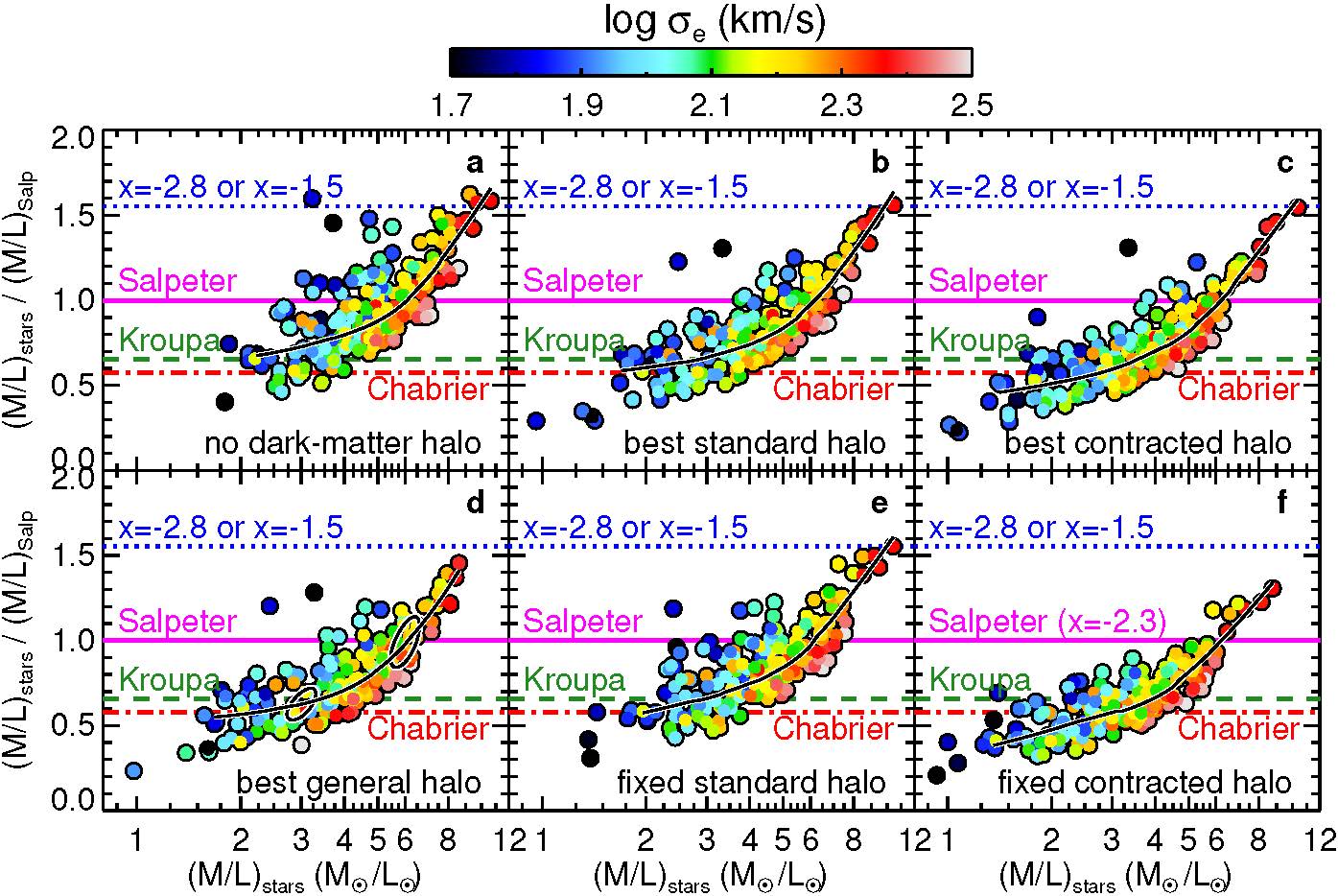 |
Figure 16. Systematic variation of the stellar IMF in ETGs. The six panels show the ratio between the (M / L)stars of the stellar component, determined using dynamical models, and the (M / L)Salp of the stellar population, measured via stellar population models with a Salpeter IMF, as a function of (M / L)stars. The black solid line is a LOESS non-parametric regression to the data. Colours indicate the galaxies' stellar velocity dispersion, σe, which is related to the galaxy mass. The horizontal lines indicate the expected values for the ratio if the galaxy had (i) a Chabrier IMF (red dash-dotted line); (ii) a Kroupa IMF (green dashed line); (iii) a Salpeter IMF (x = -2.3, solid magenta line) and two additional power law IMFs with (iv) x = -2.8 and (v) x = -1.5 respectively (blue dotted line). Different panels correspond to different assumptions for the dark matter halos employed in the dynamical models as written in the black titles. A curved relation is clearly visible in all panels. From Cappellari et al. (2012). |
The most extensive set of detailed dynamical models to date, accurately reproducing both the galaxy photometry and the integral-field stellar kinematics, was constructed for the 260 ETGs of the ATLAS3D survey (Cappellari et al. 2013b). This study used axisymmetric anisotropic models based on the Jeans equations (JAM in Section 5.3.3) and includes a rather general dark halo, where both its slope and normalization are varied to reproduce the data within a Bayesian framework. The halo inner logarithmic slope is allowed to vary from the values predicted by halo contraction models (Abadi et al. 2010) to the nearly constant density profiles expected from halo expansion models (Pontzen & Governato 2012). The median fraction of dark matter inferred from the models, within a sphere of radius r = Re, is just 10-20%. Cappellari et al. (2013b) find this dark matter fraction to be consistent with predictions for the same galaxies inferred by linking NFW halos to the real galaxies and assuming halo masses via the halo abundance matching technique (e.g. Behroozi et al. 2010). Using satellites as tracers of the gravitational potential, the NFW model of Wojtak & Mamon (2013) extrapolates 18 to a similar DM fraction within Re for red galaxies of masses 1.6 - 5 × 10¹¹ M⊙ (see Figure 17 below), but to much larger dark matter fractions for lower and higher mass red galaxies.
The study of Cappellari et al. (2012) finds that dark matter cannot explain the systematic increase in the total M / L with the galaxies velocity dispersion σe. This implies a systematic variation of the stellar IMF with σe, with the mass normalization changing by a factor up to 2-3, or from Chabrier (2003) or Kroupa (2001) to heavier than Salpeter (1955) over the full galaxy population (Figure 16; Cappellari et al. 2012). The Salpeter or heavier IMF for the most massive ETGs is consistent with recent findings from the analysis of IMF sensitive spectral features (van Dokkum & Conroy 2010; Spiniello et al. 2012; Conroy & van Dokkum 2012) and with strong lensing results (see, e.g., Treu et al. 2010; Auger et al. 2010b; Dutton et al. 2013, and discussion in Section 7), under the assumption of cosmologically motivated dark matter halos. This result also smoothly bridges the gap between the IMF inferred for massive ETGs and the lighter Chabrier/Kroupa inferred for spiral galaxies (Bell & de Jong 2001, see Section 3).
Alternatives to a non-universal IMF do exist, to explain the dynamical or lensing results, but they require that (i) either all current stellar population models (Section 2) systematically and severely under predict the M / L for the galaxies with the largest σ, which are characterized by the largest metallicities, or (ii) the dark matter accurately follows the stellar distribution, contrary to what all simulations predict. Moreover the IMF trends inferred from spectral absorption features would need to be explained by a conspiracy of chemical abundance variation with galaxy σ. There is currently no evidence for any of these effects, but further investigations in these directions are still important.
Several recent studies have provided kinematic measurements of the integrated stellar light of ETGs beyond 3-4 Re, using long-slit (Thomas et al. 2007; Proctor et al. 2009; Coccato et al. 2010; Arnold et al. 2011) or two-dimensional spectroscopy (Weijmans et al. 2009). This, however, remains a rather challenging task, and as we probe outwards we must consider more discrete tracers such as globular clusters and planetary nebulae (see Section 5.5.2 below). The results obtained so far have provided a picture where ETGs are dominated by the stellar mass out to 1-3 Re, thus playing the counterpart of the maximum disk hypothesis in gas-rich systems (see Section 3.4.1) but for hotter stellar systems, while the outer halos are generally consistent with ΛCDM predictions.
5.5.2. Globular Clusters and Planetary Nebulae: the Outer Regions
In order to probe the distant radii beyond ≃ 4 Re, observations from individual globular clusters (e.g. Foster et al. 2011) or planetary nebulae (Douglas et al. 2007; Romanowsky et al. 2009; Coccato et al. 2009; Napolitano et al. 2011) become essential, even though these populations are often scarce. See Gerhard (2013) for a recent review.
Globular clusters (GCs) have been used extensively to probe the mass distribution of the outer halos of ETGs (see e.g. Côté et al. 2003; Hwang et al. 2008; Lee et al. 2010, and references therein). There are three drawbacks to adopting GCs as dynamical tracers. 1) As most GCs are red and very old, they have orbited many times around their host galaxy, and the most adventurous ones with the smallest pericentres will have been progressively tidally stripped by the potential of the host galaxy. Therefore, for a given apocentre, the GCs with the largest pericentres will have survived, leading to a bias towards more circular orbits (in comparison with the underlying stellar population). 2) Their dynamics is thought to originate from rather violent physical processes (early collapse, gas-rich mergers) and may therefore not be strictly linked with the orbital structure of the old stellar population (Bournaud et al. 2008). 3) A bimodality in the colour distribution of GCs in bright ETGs is often observed (Brodie & Strader 2006), which may then call for several decoupled dynamical components in the final modelling. As for any tracer embedded in the outermost regions of a galaxy potential, it is sometimes difficult to assess the steady-state and dynamically relaxed nature of a certain tracer, and address whether or not the observations still probe the galaxy potential or lie beyond the boundary with the intra-cluster potential (Doherty et al. 2009).
One of the most thorough studies of a GC system by Schuberth et al. (2010) includes nearly 700 GCs for the central Fornax cluster massive early-type galaxy NGC 1399. Using a β = Cst Jeans analysis, these authors showed that the red GC population traces very well the field stellar population, while the blue one appears to be the superposition of several sub-populations including accreted or true cluster members. A similar study of the same galaxy with (4 times fewer) PNe by McNeil et al. (2010) illustrates the relative merits of using GCs and PNe as tracers of the gravitational potential.
It is fortunate that planetary nebulae (PNe) do not suffer from the three drawbacks affecting GCs. PNe are generally thought to represent the distribution and dynamics of the galactic stellar halos with high fidelity (see, however, Méndez et al. 2001; Sambhus et al. 2006). Moreover, they are easy to observe, especially thanks to their very strong [OIII] emission line at 5007 Å. Henceforth, several dynamical studies have targeted PNe around bright ETGs using multi-slit or slit-less spectroscopy, or with the dedicated Planetary Nebulae Spectrograph (Douglas et al. 2002).
First analyses (Méndez et al. 2001; Romanowsky et al. 2003; Douglas et al. 2007) based on Jeans analysis and Schwarzschild modeling suggested that the host galaxies studied lacked DM, and were consistent with no DM (Romanowsky et al. 2003). However, recent results (e.g. Das et al. 2011) strongly confirm and quantify the discrepancy between the observed dynamics and that expected from the sole stellar light in giant ETGs such as NGC 4649. The extracted PNe luminosity distribution has also served to improve the distance estimated to that galaxy (Teodorescu et al. 2011). Although PN-based kinematic modeling is usually limited by the number of tracers (typically 100 to 200), the PN.S team has performed an ambitious observational program observing PNe in the outer regions of a dozen ETGs, with detailed results on a number of prototypical systems such as NGC 4374 in the Virgo cluster, reaching out to ≃ 5 Re (Napolitano et al. 2011). This kinematic modeling usually assumes spherical symmetry, but there now exist several studies using axisymmetric models: e.g. NGC 4494 (Napolitano et al. 2009), NGC 3379 (de Lorenzi et al. 2009), NGC 4697 (Das et al. 2011).
The main limitation of such studies is the often assumed hypothesis of spherical symmetry for the mass distribution, but these results can still serve as strong guidelines to constrain the presence of dark matter in the outer halos of ETGs.
5.5.3. Other Tracers and Combined Approaches
At such large radii reached by the GC populations, as in NGC 1399, many studies take advantage of the presence of large X-ray halos around specific ETGs to constrain the corresponding radial mass, and make direct comparisons (Humphrey et al. 2006; Schuberth et al. 2010; Das et al. 2011; Gerhard 2013). A number of galaxies have been surveyed, mostly massive ETGs as they are more often embedded within such X-ray halos (Fukazawa et al. 2006; Nagino & Matsushita 2009). The assumed hypothesis of hydrostatic equilibrium for the hot gas may sometimes hamper the robustness of such conclusions, but these effects are generally thought to be small. This is convincingly confirmed by comparing several concomitant tracers (Churazov et al. 2008; Humphrey & Buote 2010; Humphrey et al. 2011) though some discrepancies have been reported, sometimes suggesting a transition from the galaxy halo to the cluster intergalactic medium (Schuberth et al. 2010), or sometimes not yielding firm conclusions on their origins (Romanowsky et al. 2009).
As also mentioned above, even ETGs have sufficiently abundant (and well-behaved) gas components that can be used to constrain mass profiles out to large radii (Franx et al. 1994; Weijmans et al. 2008).
Orbits of individual satellites may further help constraining the potential around a galaxy (Geehan et al. 2006; van der Marel & Guhathakurta 2008). Prada et al. (2003) and Klypin & Prada (2009) used the SDSS to stack the PPS built from the satellites of thousands of otherwise fairly isolated galaxies and found it to be consistent with the predictions of ΛCDM simulations. Conroy et al. (2007) and More et al. (2011b) analysed galaxy satellites based on SDSS data, and derived the variation of virial mass with host galaxy luminosity, separating red and blue galaxies. They found both that red host galaxies of given blue luminosity have typically double the halo mass as their blue counterparts of same stellar mass. These two studies make assumptions that thwart the derivation of useful constraints on the anisotropy. Using the ΛCDM halo DF model (Wojtak et al. 2009) on a larger SDSS sample, Wojtak & Mamon (2013) are able to obtain more reliable relations between halo and stellar mass or luminosity, confirming to first order the results of Conroy et al. and More et al.. The stellar fractions within the virial radius of red galaxies with logMstars > 10 exceed 1%, peaking at 2% for logMstars ≈ 11.9 and decreasing again to 1% at larger masses. However, Wojtak & Mamon also find that red galaxies have more concentrated halos than blue galaxies of same stellar or halo mass, and that the orbits of satellites are marginally radial in the central regions, and increasingly radial with distance to the center. The reader may consult sections Section 6 and Section 7 on lensing for further details about the galaxy mass profiles at large radii.
As hinted above, a promising path toward robust mass profiles comes from the simultaneous use of all available tracers, hoping for a consistent picture to emerge. Many studies have been conducted towards this end, mostly targeting ETGs (Foster et al. 2011) and more specifically very massive ones (Woodley et al. 2010; Das et al. 2011; Arnold et al. 2011; Murphy et al. 2011). In agreement with results stated above, the overall impression from these studies calls for ETGs as being dominated by baryons within 1 Re, with DM representing about half of the mass within 2-4 Re and dominating at larger radii.
5.5.4. The Mass-Anisotropy Degeneracy
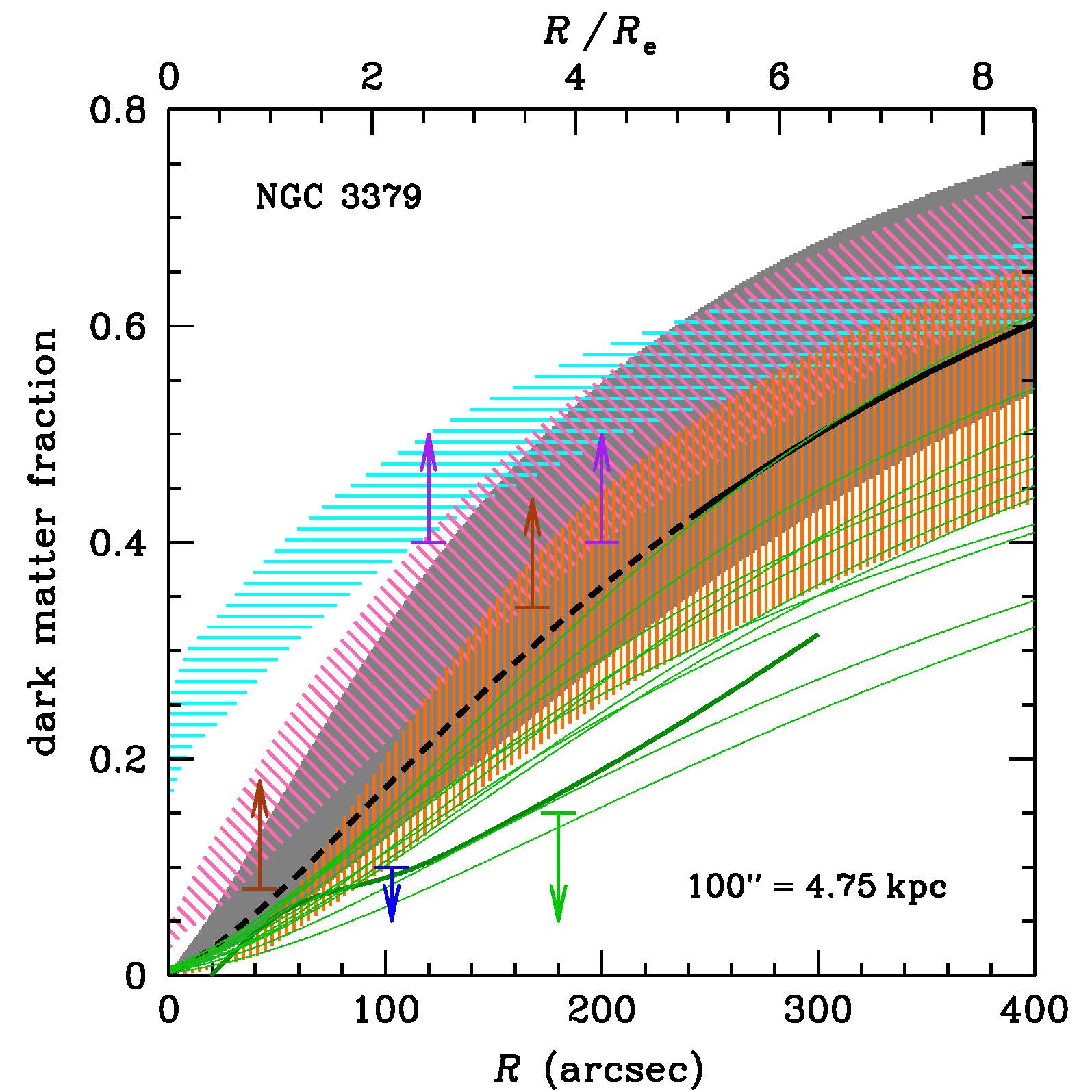 |
Figure 17. Dark matter fraction versus physical radius in NGC 3379 (assuming Re = 47" and Sérsic index n = 4.74, following Douglas et al. 2007). The light green upper limit and light green curves respectively show the Jeans (PNe) and orbit-modelling solutions of Romanowsky et al. (2003) (stars+PNe), while the blue upper limit is the DF-modelling (stars) of Kronawitter et al. (2000). The medium-thickness dark green curve shows the spherical Jeans solution (stars+PNe) with double the number of PNe Douglas et al. (2007). The orange vertically-shaded region gives the limits of NMAGIC orbit-modelling (stars+PNe) de Lorenzi et al. (2009). The lower limits shows the orbit-modelling (stars) by Weijmans et al. (2009) (brown) and the isotropic Jeans analysis (globular clusters) of Pierce et al. (2006) (purple). The cyan horizontal- and magenta oblique-shaded regions give the predictions (see Dekel et al. 2005) from equal-mass merger SPH+cooling+feedback simulations (Cox et al. 2004), of respectively gas-poor and gas-rich spirals embedded in dark matter halos. The black curve is from the satellite kinematics study of Wojtak & Mamon (2013), adopting the mean of their 3rd and 4th stellar mass bins for red hosts (the stellar mass of NGC 3379 is in between), dashes for the extrapolation within the smallest satellite radii analyzed, while the grey shaded region represents the 1 σ confidence from the Monte Carlo Markov Chain analysis of Wojtak & Mamon. |
The results presented in this section appear robust in a statistical sense. However, on an individual basis, measuring the mass profile in gas-poor galaxies is intrinsically difficult due to the degeneracy in the stellar dynamical models. The MAD is best broken by the joint use of several tracers, especially if they probe the same region of the potential. The use of tracers with very different orbital anisotropies can also be very useful to lift the MAD.
As an illustration of this MAD problem, Figure 17 shows the wide variety of solutions for the nearby (apparently) roundish ETG, NGC 3379, which had been the test-bed for the putative suggestion that ETGs are devoid of DM (Romanowsky et al. 2003; Douglas et al. 2007). One notices highly discrepant conclusions from various modeling attempts, in particular at the outer limit of spectroscopic observations (~ 200″ or ≃ 4 Re). The MAD is clearly present as the higher DM fractions indicate fairly radial orbits in the outer regions, while the lower ones come with isotropic orbits (e.g. de Lorenzi et al. 2009): this emphasizes the fact that specific tracers may constrain the mass distribution with uncertainties of different amplitude and nature. Moreover, there is a wide range of theoretical predictions. Also, some of the orbit solutions of Romanowsky et al. (2003) indicate 'normal' levels of DM at large radii (Mamon & Łokas 2005b). In fact, all recent observational modelling of NGC 3379 lead to an increased fraction of DM at increasing large radii. If NGC 3379, which has quasi-circular isophotes, were a nearly face-on S0 (Capaccioli et al. 1991), as suggested by its classification as a fast rotator (Emsellem et al. 2007), one would expect lower DM fractions (Magorrian & Ballantyne 2001).
5.5.5. Discrete Star Velocities for Dwarf Spheroidal Galaxies
Relative to giant ETGs, dSphs constitute the other mass extreme. The study of such low luminosity objects and very faint galaxies relies mostly on very nearby (Local Group) galaxies, and largely in the context of resolved stellar populations (e.g. Gilmore et al. 2007). Mass modelling is feasible thanks to ambitious observational programs to measure the stellar kinematics of hundreds and sometimes several thousands of individual stars 19 (Tolstoy et al. 2004; Łokas et al. 2005; Simon & Geha 2007; Walker et al. 2009a; Geha et al. 2010; Battaglia et al. 2011; Simon et al. 2011). We refer the reader to the detailed review by Battaglia et al. (2013).
An example of this method is shown in Figure 18 for the Sculptor dwarf spheroidal galaxy, studied in detail by Battaglia et al. (2008), who fit the PPS assuming Gaussian LOS velocity distributions (adding a component for contamination by our Milky Way). By disentangling the metal-poor and metal-rich stellar sub-populations, the authors were able to show that, if physically meaningful, these two sub-systems were compatible with the same potential (best fitted by an isothermal DM profile) but with different anisotropy, providing some clues about their origin, as the metal-rich sub-population appears to show a faster transition to radial orbits than the metal-poor one. The resulting dynamical mass-to-light ratio M / L reached values in excess of 150 inside ~ 2 kpc, demonstrating the dominance of DM at all radii in such low surface brightness objects. Walker & Peñarrubia (2011) use a similar 2-population analysis to constrain the slopes of the mass profiles of the Fornax and Sculptor dSph galaxies, ruling out cusps as steep as -1 (NFW) for both, and favoring inner slopes of -0.4 ± 0.4 (Fornax) and -0.5 ± 0.5 (Sculptor).
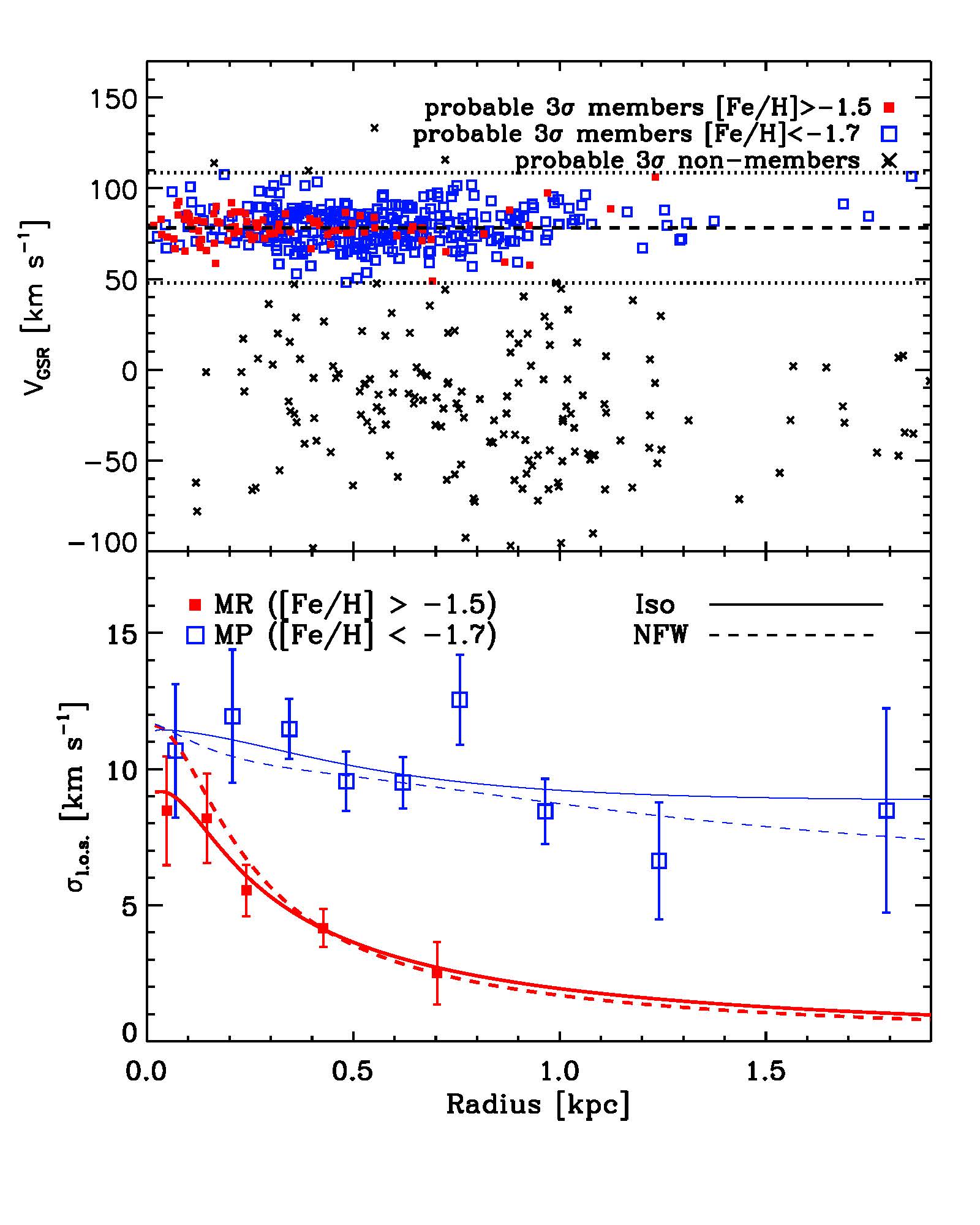 |
Figure 18. VLT/FLAMES velocity measurements for individual stars along the line-of-sight to the Sculptor dwarf spheroidal galaxy (dSph). Top panel: Line-of-sight velocities in the Galactic standard of rest versus projected radius for probable members to the Sculptor dSph (the filled and open squares show probable members with metallicity [Fe/H] > -1.5 and < -1.7, respectively) and for probable non-members (crosses). The region of probable membership is indicated by the two horizontal dotted lines, while the dashed line indicates the systemic velocity of the galaxy. Bottom panel: Line-of-sight velocity dispersion profiles for the "metal-rich" ([Fe/H] > -1.5) and "metal-poor" stars ([Fe/H] < -1.7), as shown by the filled and open squares with error-bars, respectively. The solid and dashed lines show the l.o.s. velocity dispersion profiles for the best-fitting pseudo-isothermal (cored) and NFW (cusped) dark matter models. Figure adapted from results presented in Battaglia et al. (2008). |
The DM core in Sculptor has been recently confirmed by Richardson & Fairbairn (2013b) using their new dispersion-kurtosis analysis with general anisotropy (Richardson & Fairbairn 2013a). Amorisco & Evans (2012) noted that Fornax has three distinct stellar populations (with different metallicities), and with this constraint, Amorisco et al. (2013) have shown that Fornax must indeed have a core of 1-0.4+0.8 kpc or else an NFW model with an unlikely very large scale radius. However, orbit modelling allows a cusp for Sculptor (Breddels et al. 2013) and Fornax (Jardel & Gebhardt 2012). Indeed, using orbit modelling, Breddels & Helmi (2013) conclude that while Fornax, Sculptor, Carina and Sextans can each accommodate either a cusp or a core, cores are unlikely when these 4 dSph galaxies are considered together. The debate between halo cusps and cores is thus still ongoing, largely because studies often group together different stellar populations that share different kinematics and neglect small but non-negligible rotation, and because non-spherical modelling increases the space of acceptable solutions.
Strigari et al. (2010) used an isotropic analysis (with Eq. (41) and Eddington's formula, and extracted the dispersion and kurtosis profiles from the former) to show that the classical dSph galaxies have LOS velocity dispersion, kurtosis and even distributions that are consistent with their surface density and with subhalos taken from the Aquarius ΛCDM simulation of the Milky Way (Springel et al. 2008), with dynamical masses between 2 and 15 × 108 M⊙. More generally, it is believed (see Mateo 1998, and references therein) that most dSphs have very high virial-theorem M / Ls. Recently, Walker et al. (2009b) and Wolf et al. (2010) have found that dSph M / Ls within the half-light radius increase towards lower masses down to the lowest mass ultra-faint dwarfs (UFDs). Although extrapolating these systems to their virial radii may be ill-advised, the data are consistent with all dSphs (including UFDs) having virial masses above 108 M⊙ (Walker et al.; Wolf et al.).
However, the detailed modelling of dSphs is challenging because of Milky Way contamination (e.g. Łokas et al. 2005) and because their likely tidal tails are expected to lie very close to the LOS (Klimentowski et al. 2009), which could then lead to an overestimate of their mass (Klimentowski et al. 2007).
Furthermore, when the stellar velocity dispersion reaches extremely low values, additional ingredients such as the contribution of binary systems must be taken into account for proper dynamical modelling in particular for ultra-faint dwarf galaxies (see e.g. Martinez et al. 2011, and references therein). N-body models may be required for an accurate dynamical modelling of these objects.
We have reviewed the basic methods to determine the distribution of total mass in gas-poor galaxies, whilst addressing a number of intrinsic degeneracies that may affect current determinations. We see two main directions for future applications of the discussed techniques:
One the one hand, for Local Group galaxies, the dynamical degeneracies can be alleviated by increasing the dimension of the observable space, namely by observing proper motions together with radial velocities of individual stars. At the present, this can be done for nearby star clusters by including plane-of-sky velocities from stellar proper motions in the dynamical models (e.g. van de Ven et al. 2006; van den Bosch et al. 2006; van der Marel & Anderson 2010).
The global space astrometry satellite GAIA (Perryman et al. 2001) will provide proper motions with unprecedented accuracy. Unfortunately, the classical dSph galaxies are so distant that the error on proper motions from GAIA will be of the order of their internal velocity dispersions (e.g. Battaglia et al. 2013), so the gain from proper motions with GAIA may only be significant for the closest dSph galaxies. However, the future generation of 30-40m telescopes should roughly double the GAIA precision on proper motions (with a 5-year baseline, Davies & Genzel 2010), and lead to much more accurate mass and orbital modeling (as first suggested by Leonard & Merritt 1989).
These data will require and exploit the full generality and sophistication of the models. However, it is likely that such a wealth of data will also reveal new degeneracies associated with the sub-populations of stars in galaxies, themselves reflecting their complex formation and evolution history.
Meanwhile, if the increase in computing power grows at the current rate, one should be able to increasingly resort to N-body modelling (or associated techniques) to determine the distribution of mass in ETGs and dSphs that are not in perfect dynamical equilibrium and possibly address such models in some restricted cosmological context.
On the other hand, the same simpler techniques that are being applied today to relatively small samples of nearby galaxies will be used to study much larger samples of galaxies with two-dimensional stellar (and gaseous) kinematics and at increasingly larger redshift. The current state of the art is defined by the ATLAS3D (Cappellari et al. 2011) and CALIFA surveys (Sánchez et al. 2012), which have mapped a few hundred galaxies via integral-field spectroscopy. Ongoing surveys, such as the SAMI (PI: Scott Croom) and MaNGA (PI: Kevin Bundy), will extend the sample size by about two orders of magnitude, using multi-object two-dimensional spectrographs on dedicated telescopes. Accurate masses, which themselves rely on accurate distances, will still be a critical ingredient to study galaxy formation from these larger samples. Finally, the next frontier will involve constructing dynamical models of galaxies at significant redshift, to trace the assembly of galaxy masses over time. This will also make use of multi-object spectrographs, optimized for near-infrared wavelengths, to effectively reduce the exposure times by orders of magnitude, mounted on future generation very large telescopes. Within the next ten years (i.e. ~ 2024), we may be able to approach the quality of the stellar kinematics of galaxies obtainable today in the Virgo cluster, up to the key redshift z ~ 2, when the Universe was just a quarter of its current age and much of the galaxy mass was being assembled.
8 Their expression for (M / L)(rM = Re) was converted to enclosed mass assuming (M / L)(rM = Re) ≈(M / L)(rM = r1/2). Back.
9 Churazov et al. (2010) suggested a generalization of the approach of Wolf et al. (2010) by computing the mass at the radius where mass is least dependent on anisotropy, assuming the 3 cases of isotropic, radial and circular orbits. Back.
10 The aperture velocity dispersions generally involve a triple integral. However, for simple anisotropic velocity models, one-third times the denominator of Eq. (28) becomes ∫0Rσ R dR ∫R∞ Kβ(r / R, ra / R) ν(r) M(r) dr / r, where Kβ is a dimensionless kernel given in Mamon & Łokas (2005b). Back.
11 At r200, the mean mass density is defined to be 200 times the critical density of the Universe. Back.
12 The virial radius is defined to be that where the radial streaming motions are small, typically 4/3 of r200. Back.
13 This should never be assumed but rather demonstrated. Back.
14 The Jeans equations are also called "equations of stellar hydrodynamics" or "hydrostatic equations". Back.
15 Walker et al. (2009b) did not fit the PPS but σlos(R). Back.
16 See also the use of low-mass X-ray binaries as mass/dynamical tracers in dSph galaxies by Dehnen & King (2006). Back.
17 The more rapidly declining surface brightness profiles of dwarf ellipticals relative to their giant counterparts makes the spectroscopic measurements at several Re especially challenging. Back.
18 The projected radii of the satellite galaxies analyzed by Wojtak & Mamon (2013) begin at 5 Re. Back.
19 Similar methods apply to the study of Milky Way stars; see Section 4. Back.