Bright red giant stars are detectable as point sources with mV ≲ 21 mag out to distances of ∼ 0.5 Mpc. Within this range, the Milky Way's dSph galactic satellites appear as localised overdensities of individually resolved stars. Empirical information about the number, stellar structure and internal kinematics of these systems has steadily accumulated for the past eight decades.
Shapley (1938a) discovered the Sculptor dSph upon visual examination of a photographic plate exposed for three hours with the 24-inch Bruce telescope at (what was then) Harvard's Boyden observatory in South Africa. In this original dSph discovery paper, Shapley notes that Sculptor is visible — in hindsight — as a faint patch of light on a plate taken for the purpose of site testing, in 1908, during a series of five exposures totalling nearly 24 hours with a 1-inch refracting telescope.
Reporting shortly thereafter the similar discovery of Fornax, Shapley (1938b) notes that the new type of ‘Sculptor-Fornax’ cluster shares properties with both globular clusters and elliptical galaxies, then speculates that ‘At the distance of the Andromeda system these objects would, in fact, have long escaped discovery. There may be several others in the Local Group of galaxies; such objects may be of frequent occurence in intergalactic space and of much significance both in the census and the genealogy of sidereal systems.’
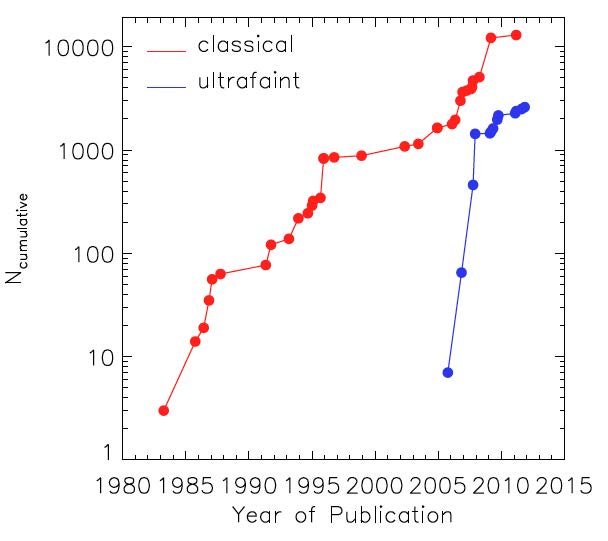
Figure 1 demonstrates Shapley's prescience, plotting the cumulative number and luminosities of the Milky Way's known dSph satellites against date of discovery publication. Harrington & Wilson (1950) and Wilson (1955) found the next four ‘Sculptor-type’ (as they were then called) systems — Leo I, Leo II, Draco and Ursa Minor — on photographic plates taken for the Palomar Observatory Sky Survey with the 48-inch Schmidt telescope. Cannon et al. (1977) spotted Carina by eye on a plate taken with the 1.2-meter UK-Schmidt Telescope. Irwin et al. (1990) used the Automated Photographic Measuring (APM) facility at the University of Cambridge to detect Sextans, again on a UK-Schmidt plate, thereby completing the census of the Milky Way's eight so-called ‘classical’ dSphs.
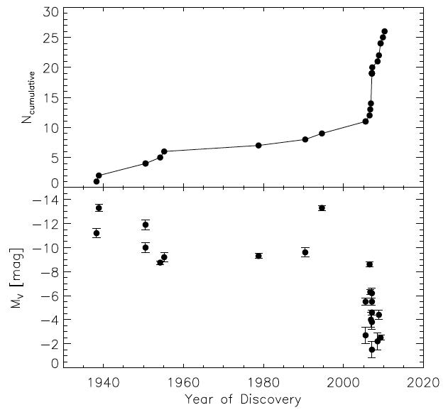 |
Figure 1. Cumulative number (top) and luminosity (bottom) of known dwarf spheroidal satellites of the Milky Way, versus year of publication of discovery paper (Shapley, 1938a, b, Harrington & Wilson, 1950, Wilson, 1955, Cannon et al., 1977, Irwin et al., 1990, Ibata et al., 1994, Willman et al., 2005b, a, Belokurov et al., 2006, Zucker et al., 2006b, a, Belokurov et al., 2007, Irwin et al., 2007, Walsh et al., 2007, Belokurov et al., 2008, Belokurov et al., 2009, Grillmair, 2009, Watkins et al., 2009, Belokurov et al., 2010). |
The next discovery was unique in that it came via spectroscopy rather than imaging. During a stellar kinematic survey of the Galactic bulge, Ibata et al. (1994) noticed Sagittarius (Sgr) in color-velocity space as an excess of stars following a narrow velocity distribution offset from that of bulge members. Subsequent observations showed that Sgr, located just ∼ 15 kpc behind the Galactic center, spews stars along tidal tails that wrap spectacularly around the entire sky (e.g., Mateo et al. 1996, Ibata et al. 1997, Majewski et al. 2003, Belokurov et al. 2006, Koposov et al. 2011a). The tidal disruption of Sgr provides a useful tracer of the Galactic potential (e.g., Johnston et al. 2005, Law & Majewski 2010, Peñarrubia et al. 2010), but disqualifies Sgr from a simple equilibrium-dynamical analysis. For this reason Sgr shall not be considered further here.
In a span of seven years, deep multi-color photometry from the Sloan Digital Sky Survey (SDSS) has now tripled the number of known Milky Way satellites (Willman et al., 2005b, a, Zucker et al., 2006b, a, Belokurov et al., 2006, Belokurov et al., 2007, Irwin et al., 2007, Walsh et al., 2007, Belokurov et al., 2008, Belokurov et al., 2009, Grillmair, 2009, Watkins et al., 2009, Belokurov et al., 2010). The 17 satellites discovered with SDSS data have extended the floor of the observed galaxy luminosity function from MV ≳ −8 to MV ≳ −2 (bottom panel of Figure 1), such that some galaxies are less luminous than some stars! Unlike their brighter ‘classical’ siblings, the ‘ultrafaint’ satellites 1 discovered with SDSS data are not apparent to the eye, even in deep images. Rather, they are detected only by correlating spatial overdensities with overdensities in color-magnitude space (e.g., Belokurov et al. 2006, Walsh et al. 2009). In order to confirm the faintest satellites, the SDSS catalog must be supplemented by deeper, follow-up photometry as well as spectroscopy (e.g., Belokurov et al. 2009, 2010). Given the rate of false positives expected for candidates remaining in SDSS data (≳ 4/5 in the author's experience), the expense of follow-up observations can be prohibitive. However, the next generation of sky surveys (Pan-STARRS, SkyMapper, DES, Gaia, LSST, etc.) will almost certainly bring a new flurry of discoveries, particularly in the relatively unexplored southern sky.
Although they are not considered further below, it is worth noting that Shapley was correct regarding the dSph satellites of M31. van den Bergh (1972) discovered the first example with the Palomar Schmidt telescope, using plates more sensitive than those used in the original Palomar Survey. The current census includes 27 known dSph satellites of M31. Two-thirds of this number were discovered in the past seven years (Zucker et al., 2004, Martin et al., 2006, Ibata et al., 2007, Zucker et al., 2007, Majewski et al., 2007, Irwin et al., 2008, McConnachie et al., 2008, Martin et al., 2009, Richardson et al., 2011, Slater et al., 2011, Bell et al., 2011), with SDSS data as well as photometry from the PAndAS survey conducted with the Canada-France-Hawaii Telescope (McConnachie et al., 2009).
Galactic dynamics is concerned with the relationship between gravitational potential and the distribution of stars in phase space. Observers who study dark matter in dSph galaxies must gather information about the positions and velocities of dSph stars. The largest dSphs subtend solid angles of several square degrees, making it difficult to study their stellar structure at large radius. Complete homogenous surveys are rare and valuable.
Hodge (1961b, a, 1962, 1963, 1964a, b) used photographic plates obtained at the Palomar (48-inch Schmidt, 100-inch and 200-inch), Lick (120-inch) and Boyden Station (24-inch Schmidt) in order to study luminous structure of the six Milky Way dSphs known at the time (Sculptor, Fornax, Leo I, Leo II, Draco and Ursa Minor). Hodge counted stars within squares of regular grids overlaid on each plate, and provides this description of analog data reduction: ‘Each plate was counted at one sitting so that uniformity would be maintained. The plates were counted to the limiting magnitude and each was counted once. From experience ... it was decided that the reproducibility of counts on a particular plate is greater than from plate to plate, so that it is better to count many plates each once than one plate many times’ (Hodge, 1961b).
Figure 2 (top two rows of panels) displays isopleth maps that Hodge drew by connecting squares containing equal numbers of stars. These maps reveal that the internal structure of dSphs is smooth. Hodge reasoned that a well-mixed dSph requires dynamical relaxation by a process other than stellar encounters, as the low surface densities of dSphs imply internal relaxation timescales of ≳ 103 Hubble times. Hodge (1966) and Hodge & Michie (1969) would later suggest that encounters between stellar groups might enable exchanges of orbital energy over shorter timescales during dSph formation. Eventually Lynden-Bell (1967) would show that the time-varying gravitational potential of a young galaxy effectively shuffles the orbital energies of its stars, generating ‘violent’ relaxation without stellar encounters. More recently, Mayer et al. (2001b) have proposed a mechanism specific to dSphs, demonstrating with N-body/hydrodynamical simulations that repeated tidal encounters with the Milky Way can effectively transform a rotating dSph progenitor into a pressure-supported spheroid in less than a Hubble time.
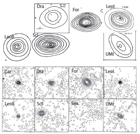 |
Figure 2. Stellar isodensity maps for the Milky Way's eight ‘classical’ dSphs. Top two rows: from Hodge's star count studies (Hodge, 1961b, a, 1962, 1963, 1964a, b, reproduced by permission of the American Astronomical Society). Bottom two rows: reproduced from Structural Parameters for the Galactic Dwarf Spheroidals, by M. Irwin & D. Hatzidimitriou, MNRAS, 277, 1354, 1995 (by permission of John Wiley & Sons Ltd.). |
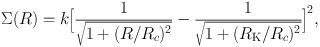
Hodge discovered two other structural features common to the classical dSphs. First, most exhibit flattened morphology, with typical ellipticities of є ≡ 1 − b / a ∼ 0.3, where a and b are semi-major and semi-minor axes, respectively. Second, dSph stellar density profiles decline more steeply at large radius than do the profiles of giant elliptical galaxies. Whereas the latter are commonly fit by formulae with relatively shallow outer profiles, e.g., Σ(R) = Σ(0) / (1 + R / a)2 (Hubble, 1930) or Σ(R) = Σ(0)exp[− kR1/4] (de Vaucouleurs, 1948), Hodge found that classical dSphs all have steeper outer profiles that are better fit with the formula of King (1962):
 |
(1) |
where Rc is a ‘core’ radius and RK is a maximum, or ‘limiting’ radius that one might expect to result from tidal truncation (Section 2.2.3) 2.
Three decades later, Irwin & Hatzidimitriou (1995, ‘IH95’ hereafter) used the APM facility at Cambridge to count stars automatically on photographic plates from the Palomar and UK Schmidt telescopes. While confirming Hodge's findings, IH95 produced significantly deeper maps and were able to include Carina and Sextans, the two Milky Way dSphs discovered in the interim (Figure 2). IH95 used these maps to measure the centroid, ellipticity and orientation of each dSph, and then to tabulate stellar density as a function of distance along the semi-major axis. While the homogeneous analysis of IH95 continues to provide a valuable resource particularly for comparing dSphs in the context of scaling relations (Section 5), deeper photometric data sets now exist for most of the classical dSphs (e.g., Stetson et al., 1998, Majewski et al., 2000, Saviane et al., 2000, Odenkirchen et al., 2001, Palma et al., 2003, Walcher et al., 2003, Lee et al., 2003, Tolstoy et al., 2004, Coleman et al., 2005a, b, Battaglia et al., 2006, Westfall et al., 2006).
In principle the structure of dSph stellar components carries information about the mechanisms that drive dSph formation and evolution. While incompatible with shallow Hubble and de Vaucouleurs profiles, the available data often do not distinguish the King profile (Equation 1) from other commonly adopted fitting formulae — e.g., exponential and Plummer (1911) profiles,
 |
(2) |
and
 |
(3) |
respectively, where Rh ≈ 1.68Re is the projected halflight radius (i.e., the radius of the circle enclosing half the stars as viewed in projection). Figure 3 displays IH95's fits of King (1966) and exponential surface brightness profiles to the Milky Way's classical dSph satellites.
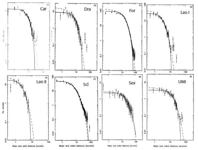 |
Figure 3. Stellar density profiles for the Milky Way's ‘classical’ dSphs. Overlaid are best-fitting King (1966, solid) and exponential (dashed) surface brightness profiles. Reproduced from Structural Parameters for the Galactic Dwarf Spheroidals, by M. Irwin & D. Hatzidimitriou, MNRAS, 277, 1354, 1995 (by permission of John Wiley & Sons Ltd.). |
The SDSS catalog enables homogeneous studies of the structural properties of ultrafaint dSphs. For example, Figure 4 displays isopleth maps constructed by Belokurov et al. (2007) for Coma Berenices, Canes Venatici II, Segue 1 and Hercules using both SDSS and deeper follow-up data. Whereas Hodge and IH95 estimated structural parameters for the classical dSphs after binning their star-count data and subtracting estimates of foreground densities, the low surface brightnesses of ‘ultrafaint’ dSphs are conducive neither to binning nor to foreground subtraction. Fortunately, neither procedure is necessary; indeed Kleyna et al. (1998) estimate structural parameters for the classical dSph Ursa Minor using a likelihood function that specifies the probability associated with each individual stellar position in terms of a parametric surface brightness profile plus constant foreground.
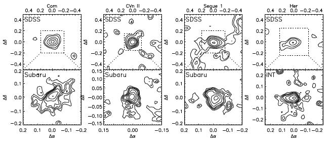 |
Figure 4. Stellar idodensity maps for four of the Milky Way's ‘ultrafaint’ dSphs, from the discovery paper of Belokurov et al. (2007, reproduced by permission of the American Astronomical Society). |
Martin et al. (2008) design a similar maximum-likelihood analysis that operates directly on unbinned SDSS data in order to estimate the centroid, halflight radius, luminosity, ellipticity and orientation of each ultrafaint satellite. Figure 5 demonstrates the efficacy of their method. The left panel maps individual stars from the SDSS catalog that are near the line of sight to Boötes I and satisfy color/magnitude criteria designed to select red giants at the distance of Boötes I. Panels on the right-hand side show maximum-likelihood estimates of each free parameter. Marginalised error distributions include the effects of sampling errors and parameter covariances, and can be used directly in subsequent kinematic/dynamical analyses (Section 4).
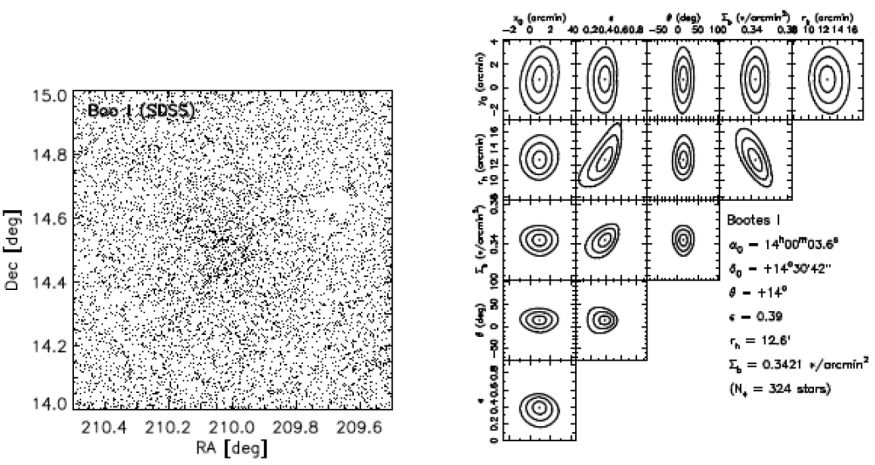 |
Figure 5. Measurement of structural parameters for the Boötes I dSph from SDSS data (Martin et al., 2008). Left: sky positions of red giant candidates selected from the SDSS catalog. Right: constraints on structural parameters, from the maximum-likelihood analysis of Martin et al. (2008, reproduced by permission of the American Astronomical Society). |
Martin et al. (2008) show that their method recovers robust estimates even when the SDSS sample includes as few as tens of satellite members. Subsequent tests with synthetic data by Muñoz et al. (2011) provide reason for caution, suggesting that for objects with low surface brightness, insufficient contrast between members and foreground can generate biased estimates of structural parameters. It is reassuring that deeper observations with CFHT (Muñoz et al., 2010) and Subaru (Okamoto et al., 2012) yield structural parameters for subsets of ultrafaint satellites that agree well with the SDSS-derived estimates of Martin et al. (2008).
The outer stellar structure of a given dSph is determined by some combination of formation processes and subsequent evolution within the external potential of the Milky Way. In his structural analyses of the six dSphs known in the 1960s, Hodge compared the observed limiting radii, RK (Equation 1), to simple estimates of ‘tidal’ radii, rt, beyond which stars escape into the external potential of the Milky Way (von Hoerner, 1957, King, 1966):
 |
(4) |
Here, MMW and MD are the Milky Way and dSph (point) masses, respectively, RD is the pericentric distance of the dSph's orbit and e is orbital eccentricity. Assuming circular orbits and considering only luminous masses, Hodge (1966) noticed that while the two radii are similar for the nearest dSphs (Draco, Sculptor, Ursa Minor), for the three most distant dSphs (Leo I, Leo II, Fornax), RK ≲ 0.5 rt. Hodge (1966) concluded that tidal forces play a significant role in shaping the outer structures of the nearest dSphs.
Low surface brightness in the outer regions of dSphs makes extended structural studies difficult to conduct and interpret. For example, Coleman et al. (2005a) use deep wide-field photometry to conclude that Sculptor's surface brightness profile is well described as the superposition of two equilibrium stellar components with different scale radii. Using an independent data set, Westfall et al. (2006) fit a single profile and identify a ‘break’ in Sculptor's surface brightness profile, which makes an apparent transition from a King profile in the inner parts to a shallower power law in the outer parts. Westfall et al. (2006) cite this transition not as evidence for a second component, but rather as a signal that Sculptor is losing stars to tidal disruption.
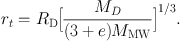
In many cases, the use of narrow-band filters that are sensitive to stellar surface gravity (e.g., DDO51) can help to distinguish dSph red giants from foreground dwarf stars, providing a valuable boost in contrast (e.g., Majewski et al., 2000, 2005, Palma et al., 2003, Westfall et al., 2006). Having used narrow-band photometry to select spectroscopic targets at large dSph radi, Muñoz et al. (2005) and Muñoz et al. (2006) present velocities that confirm the membership of stars in Ursa Minor and Carina (Figure 6) out to radii ∼ 3 and ∼ 5 times larger, respectively, than estimates of RK. These detections imply that tides can play a significant role in shaping the outer parts of dSphs (Section 3.2).
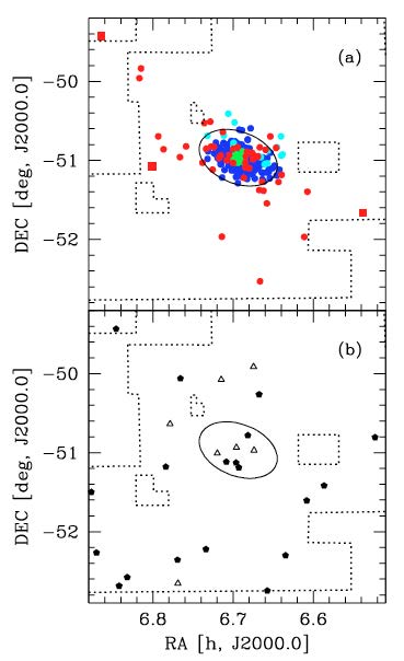 |
Figure 6. Extended stellar structure of the Carina dSph, from narrow-band photometry and spectroscopy of Muñoz et al. (2006, reproduced by permission of the American Astronomical Society). The top/bottom panels show sky positions of red giant candidates confirmed as Carina members/nonmembers. Ellipses mark Carina's limiting radius, RK (Equation 1), determined from smooth fits to star count data. The extension of faint stellar structure at R ≳ 3RK suggests tidal interaction (Section 3.2). Muñoz et al. (2005) report similar results for Ursa Minor. |
2.2.4. Structural Peculiarities of Individual dSphs
Most kinematic analyses of dSphs proceed from the assumption that dSphs host a single, spherically symmetric stellar component in dynamic equilibrium (Section 4). However, real dSphs are all flattened (0.1 ≲ є ≡ 1 − b / a ≲ 0.7, Irwin & Hatzidimitriou (1995), Martin et al. (2008), Sand et al. (2011)), and it is not clear how severely this violation of spherical symmetry affects conclusions regarding dSph dynamics. In fact most dSphs exhibit individual peculiarities that further violate the simplistic assumptions (Section 4) employed in kinematic analyses.
For example, Sculptor, Fornax and Sextans all display evidence for chemo-dynamically independent stellar sub-populations (Tolstoy et al., 2004, Battaglia et al., 2006, Battaglia et al., 2011, respectively). In all three cases, a relatively metal-rich, kinematically cold population has smaller scale radius than does a metal-poor, kinematically hot population (Section 4.2.2, Figure 10). Fornax also has irregular stellar structure in the form of a crescent-shaped feature near its center (Stetson et al., 1998, and Figure 7, left panel), two shell-like features (Coleman et al., 2004) and lobes along its morphological minor axis (Coleman et al., 2005b, and Figure 7, right panel). These features suggest that Fornax may have undergone a recent merger, an event that might be related to the presence of a young (age ∼ 100 Myr), centrally concentrated main sequence in Fornax (Battaglia et al., 2006). Ursa Minor exhibits clumpy stellar substructure, most dramatically in the form of a secondary peak in its luminosity distribution, offset by ∼ 20′ from the central peak (Olszewski & Aaronson, 1985). The region near the secondary peak is kinematically colder than the rest of Ursa Minor (Kleyna et al., 2003), and so may represent a bound star cluster (Section 4.2.1).
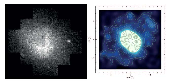 |
Figure 7. Structural irregularities in Fornax. Left: Grayscale map (∼ 42′ per side) of surface density of stars with 18.5 ≤ V ≤ 23, from the photometry of Stetson et al. (1998, reproduced with permission from The University of Chicago Press). Notice the crescent-like feature near the center. Right: Smoothed stellar map from V, I photometry of Coleman et al. (2005b, reproduced by permission of the American Astronomical Society), who detect two shell-like features (one is visible ∼ 1.3 deg northwest of the center) aligned with lobes along the morphological minor axis. |
Such peculiarities extend to the ultrafaint satellites as well. Spectroscopic surveys reveal that Segue 1 is superimposed on at least one stream of stellar debris (Geha et al., 2009, Niederste-Ostholt et al., 2009, Simon et al., 2011), offset by ∼ 100 km s−1 from Segue 1 in velocity space. Segue 1 also shows hints of extended stellar structure superimposed on Sgr debris, although interpretation of these extremely low-surface-brightness features in terms of tidal disruption remains controversial (Belokurov et al., 2007, Geha et al., 2009, Niederste-Ostholt et al., 2009, Simon et al., 2011). Segue 2 appears to be embedded in — and comoving with — a stream of stellar debris, perhaps from a tidally disrupted parent system (Belokurov et al., 2009). Ursa Major II has flattened morphology and distorted outer morphology that suggest ongoing tidal disruption (Zucker et al., 2006a, Muñoz et al., 2010). Another strong candidate for disruption is Boötes III, which has irregular, clumpy morphology and a large measured velocity dispersion of σ∼ 14 km s−1 (Carlin et al., 2009). The alignment of stellar distortions in Leo IV and Leo V hints at a low surface brightness ‘bridge’ spanning the ∼ 20 kpc between these systems (Belokurov et al. (2008), Walker et al. (2009a), de Jong et al. (2010); note, however, that Sand et al. (2010) detect no such feature in deep photometry around Leo IV). Stars nearest the center of the Willman 1 satellite exhibit near-zero velocity dispersion and a mean velocity that is offset from the rest of Willman 1 members by ∼ 8 km s−1 (Willman et al., 2011). Each newly discovered galaxy seems to present a new quirk of its own.
Assuming that dSphs are purely stellar systems truncated by tidal interaction with the Milky Way, such that rt ∼ RK, Ostriker et al. (1974) applied Equation 4 to estimate the mass of the Milky Way. Inverting the calculation by assuming an isothermal Galactic halo with vcirc = 225 km s−1, Faber & Lin (1983) estimated masses of dSphs. For the nearest dSphs (Draco, Ursa Minor, Carina, Sculptor), Faber & Lin estimated mass-to-light ratios of M / LV ≳ 10 [M / LV]⊙, suggesting dSph dark matter. Faber & Lin further used their estimates to predict, via the virial theorem, values of ≳ 10 km s−1 for the internal stellar velocity dispersions of dSphs.
At the same time, Aaronson (1983) provided the first actual measurement of a dSph's internal velocity dispersion. Aaronson used the Multiple Mirror Telescope (MMT, which then consisted of six 1.8-meter mirrors working in tandem) to acquire high-resolution (R ∼ 30000) spectra for three individual carbon stars in Draco. Figure 8 displays the spectra, which were sufficient for Aaronson to measure precise line-of-sight velocities of −298.7± 0.9 km s−1 (with a follow-up measurement of −297.6 ± 0.6 km s−1), −300.2 ± 0.6 km s−1, and −279.7 km s−1. Aaronson calculated that such measurements require, at the 95% confidence level, an intrinsic velocity dispersion of σ ≳ 6.5 km s−1. 3 From dynamical arguments based on the virial theorem (Illingworth, 1976, Richstone & Tremaine, 1986, Section 4.1.1), such a large dispersion indicates a large dynamical mass-to-light ratio M / LV ≳ 30 [M / LV]⊙, confirming the prediction of Faber & Lin (1983) and indicating the presence of dark matter.
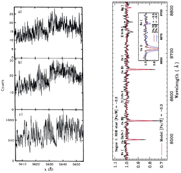 |
Figure 8. Examples of spectra for individual dSph stars. Left: MMT echelle spectra (R ∼ 30000) for three carbon stars in Draco, used for the first measurement of a dSph velocity dispersion (Aaronson, 1983, reproduced by permission of the American Astronomical Society). Right: Keck/DEIMOS spectrum (R ∼ 6000) for the brightest red giant in Segue 1 (Geha et al., 2009, reproduced by permission of the American Astronomical Society), with absorption features labeled and best-fitting model overplotted. |
Figure 9 plots the number of stars observed in dSph stellar velocity surveys as a function of time. The three decades of observations separate neatly into ‘epochs’ defined by the available instrumentation.
2.3.1. Small-Number Statistics
The 1980s yielded the first precise velocity measurements for individual stars in Draco (Aaronson, 1983), Carina, Sculptor, and Fornax (Seitzer & Frogel, 1985), Leo I and Leo II (Suntzeff et al., 1986) and Ursa Minor (Aaronson & Olszewski, 1987a), and follow-up observations of Sculptor (Armandroff & Da Costa, 1986) and Draco (Aaronson & Olszewski, 1987b). These samples typically included ≲ 10 stars per galaxy and indicated velocity dispersions of σ ∼ 6 − 10 km s−1, suggesting that dSph dynamical mass-to-light ratios reach at least double the values estimated for globular clusters. Strong implications for the particle nature of dark matter (Tremaine & Gunn, 1979, Lin & Faber, 1983, Section 6.2) drew immediate attention. Nevertheless, skepticism regarding small samples, velocity precision and the unknown contribution of binary orbital motions to the measured velocity dispersions demanded further observations and better statistics.
In the 1990s, several groups accumulated velocity samples for tens of stars per dSph. Including Aaronson's original work, nine seasons of observations with the MMT eventually produced velocity samples that reached ∼ 20 members in each of the Draco and Ursa Minor dSphs (Olszewski et al., 1995, Armandroff et al., 1995), yielding velocity dispersion measurements of σ ∼ 10 km s−1 and dynamical mass-to-light ratios M / LV ∼ 75 [M / LV]⊙ for both galaxies. Meanwhile, medium-resolution (R ∼ 12000) spectra from the William Herschel Telescope gave velocity samples for tens of stars in each of Draco, Ursa Minor and the newly discovered Sextans (Hargreaves et al., 1994b, a, 1996b). High-resolution spectra from ESO's 3.6-m and NTT telescopes (Queloz et al., 1995) and Keck/HIRES (Mateo et al., 1998) delivered precise velocities for 23 and 33 stars in Sculptor and Leo I, respectively. In all cases, velocity dispersions of σ ≳ 6 km s−1 indicated M / LV ≳ 10 [M / LV]⊙.
Providing an early demonstration of the efficiency of multi-object fiber spectroscopy, Armandroff et al. (1995) compiled samples of ∼ 100 velocities in each of Draco and Ursa Minor using the HYDRA multi-fiber spectrograph at the KPNO 4-meter telescope. This data set included many repeat measurements, which Olszewski et al. (1996) used to estimate a binary fraction of ∼ 0.2 − 0.3 for periods of ∼ 1 year. Based on Monte Carlo simulations, Olszewski et al. (1996) and Hargreaves et al. (1996a) concluded that binary motions contribute negligibly to the velocity dispersions measured for classical dSphs (Section 3.3).
In the southern hemisphere, Mateo et al. (1991) used Las Campanas Observatory's 2.5-meter telescope and ‘2D Frutti’ echelle photon counter to measure velocities for 44 Fornax stars, including an outer field that showed the same velocity dispersion (σ∼ 10 km s−1) as the central stars, indicating M / LV ∼ 10 [M / LV]⊙. After measuring a velocity dispersion of σ ∼ 7 km s−1 and M / LV ∼ 40 [M / LV]⊙ from the velocities of 17 Carina stars, Mateo et al. (1993) noted a scaling relation among dSphs: the dynamical mass-to-light ratios of classical dSphs are inversely proportional to luminosity, suggesting similar dynamical masses of ∼ 107 M⊙ (Section 5).
The gap in Figure 9 between 1998−2002 signifies a period not of inactivity but rather of construction. During this time, wide-field multi-object spectrographs were built for the world's largest telescopes. Over the past decade, surveys with these new instruments have increased stellar velocity samples from tens to thousands per dSph. Kleyna et al. (2002, 2003, 2004) used the Wide-Field Fibre Optic Spectrograph (WYFFOS) at the 2.5-meter Isaac Newton Telescope to measure velocities for ∼ 100 stars in each of Draco, Ursa Minor and Sextans, respectively. These samples were sufficiently large to examine the velocity distribution as a function of distance from the dSph center (e.g., Wilkinson et al. 2002, Kleyna et al. 2002, 2004, Wilkinson et al. 2004; Section 4).
Soon thereafter, the Dwarf Abundances and Radial Velocities Team (DART) used the FLAMES fiber spectrograph at the 8.2-meter Very Large Telescope (VLT; UT2) to measure velocities and metallicities (derived from the strength of the calcium-triplet absoprtion feature at ∼ 8500 Å) for ∼ 310, ∼ 560 and ∼ 175 members of Sculptor, Fornax and Sextans, respectively (Tolstoy et al., 2004, Battaglia et al., 2006, Battaglia et al., 2011). Theses samples yielded the discovery that all three of these dSphs contain multiple, chemodynamically independent stellar populations (Figure 10 and Section 4.2.2). Also with VLT/FLAMES, Koch et al. (2007a) measured a velocity dispersion of σ ∼ 7 km s−1 from ∼ 170 members of Leo II, providing what remains the largest published sample for this galaxy.
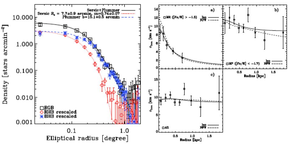 |
Figure 10. Sculptor's two chemodynamically independent stellar sub-populations (Battaglia et al., 2008, reproduced by permission of the American Astronomical Society ; see also Tolstoy et al. 2004). Left: Surface brightness profiles for Sculptor's red giants (black), red-horizontal branch (red) and blue-horizontal branch stars. Right: Velocity dispersion profiles, calculated for subsets of relatively metal-rich (top left) and metal-poor (top right), as determined from the VLT/FLAMES spectroscopic sample of Tolstoy et al. (2004). For comparison, the lower-left panel plots the velocity dispersion profile measured from the composite population. |
Meanwhile Muñoz et al. (2006) used archival VLT/FLAMES spectra (see also Fabrizio et al. (2011)) to measure velocities for ∼ 300 Carina members and added another ∼ 45 members from spectra obtained sequentially with the MIKE spectrograph at the Magellan/Clay 6.5-meter telescope. The extra members observed with MIKE extend to ∼ 5 times Carina's limiting radius as determined from photometry (Figure 6), indicating that Carina has lost mass to tidal interactions with the Milky Way.
Koch et al. (2007a) used a pair of multi-slit spectrographs — the Gemini Multiobject Spectrograph (GMOS) at the Gemini-North 8-meter telescope and the Deep Imaging Multi-object Spectrograph (DEIMOS) at the Keck 10-meter telescope — to measure velocities for ∼ 100 members of Leo I. Sohn et al. (2007) added another ∼ 100 members from their own observations with Keck/DEIMOS, and Mateo et al. (2008) contributed velocities for ∼ 300 Leo I members using the Hectochelle multi-fiber spectrograph at the MMT. The latter two studies explored larger radii and both found kinematic evidence for tidal streaming motions in the outskirts of Leo I. This result is surprising given Leo I's current distance of ∼ 250 kpc (Irwin & Hatzidimitriou, 1995), leading Mateo et al. (2008) to suggest that Leo I's orbit is nearly radial.
Operating from 2004−2011, the Michigan-MIKE Fiber Spectrograph (MMFS; R ∼ 20000), built by Mario Mateo for the Magellan/Clay 6.5-meter telescope, provided what remain the largest homogeneous velocity samples for ‘classical’ dSphs. The public catalog of Magellan/MMFS velocities includes ∼ 775, ∼ 2500, ∼ 1365 and ∼ 440 members of Carina, Fornax, Sculptor and Sextans, respectively (Walker, Mateo & Olszewski, 2009). Figure 11 displays the Fornax data, including sky positions as well as the two quantities measured from each spectrum: line-of-sight velocity and a spectral index that indicates the pseudo-equivalent width of the Mg-triplet feature at ∼ 5170 Å. Data from a similar survey conducted in the North with MMT/Hectochelle will soon become public. Figure 12 displays velocity dispersion profiles calculated from the Magellan/MMFS and MMT/Hectochelle data, demonstrating that the luminous regions of classical dSphs have approximately constant velocity dispersion.
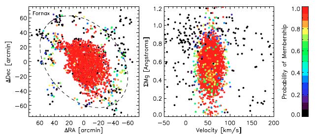 |
Figure 11. Magellan/MMFS spectroscopic data for Fornax (Walker, Mateo & Olszewski, 2009 updated to include the full sample of ∼ 3200 members). Left: Sky positions of individual stars. Right: velocities and spectral indices (pseudo-equivalent widths of the Mg-triplet absorption feature. Color indicates membership probability, as estimated from position, velocity and spectral index distributions. The ellipse indicates the limiting radius, RK (Equation 1). |
 |
Figure 12. Velocity dispersion profiles observed for the Milky Way's eight ‘classical’ dSphs (Walker et al., 2007a, Mateo et al., 2008, Walker et al., 2009b). See also Kleyna et al. (2002, 2004), Wilkinson et al. (2004), Muñoz et al. (200), 2006), Sohn et al. (2007), Koch et al. (2007b, a), Battaglia et al. (2008, 2011). Overplotted are mass-follows-light King (1966) models (Section 4.1.1) normalised to reproduce the observed central dispersions. Failure of these models to reproduce the large velocity dispersions at large radius provides the strongest available evidence that dSphs have dominant and extended dark matter halos. |
2.3.4. (Necessarily) Small Samples
With kinematic samples for ‘classical’ dSphs growing exponentially, discoveries of ‘ultrafaint’ dSphs with SDSS data generated a wave of interest in the faintest Milky Way satellites, and efforts to obtain spectroscopic follow-up began immediately. Kleyna et al. (2005) contributed a first result echoing Aaronson's original study of Draco: from Keck/HIRES velocities for 5 members of Ursa Major I, Kleyna et al. (2005) estimate that σ > 6.5 km s−1 with 95% confidence. Given UMaI's low luminosity, simple dynamical models imply M / LV ≳ 500 [M / LV]⊙. Muñoz et al. (2006) used the HYDRA multi-fiber spectrograph at the 3.5-meter WIYN telescope to measure velocities for 7 members of the Boötes I dSph, obtaining a velocity dispersion of ∼ 6.5 km s−1 and M / LV ≳ 130 [M / LV]⊙.
Whereas spectroscopic surveys of ‘classical’ dSphs target bright red giant branch (RGB) stars, the least luminous ‘ultrafaint’ satellites host few RGBs. Samples for even tens of stars for such objects require observations of faint stars near the main sequence turnoff and are feasible only with the largest telescopes. Martin et al. (2007) and Simon & Geha (2007) used Keck/DEIMOS to observe tens of velocities in 10 of the 11 ‘ultrafaints’ known at the time, measuring σ ≳3 km s−1 and concluding that these objects indeed have extremely large dynamical mass-to-light ratios, of order M / LV ≳ 100 [M / LV]⊙ and larger. Geha et al. (2009, see example spectrum in the right panel of Figure 8) and Simon et al. (2011) followed with a Keck/DEIMOS survey of Segue 1, measuring σ ∼ 4 km s−1 and concluding that this object is the ‘darkest galaxy’, with M / LV ∼ 3400 [M / LV]⊙.
Adén et al. (2009) and Koposov et al. (2011b) used VLT/FLAMES to measure velocity dispersions for Hercules and Boötes I, respectively, that while indicative of large dynamical mass-to-light ratios, are both smaller than previously measured with Keck/DEIMOS. Adén et al. (2009) obtained a smaller velocity dispersion after using Strömgren photometric criteria to remove foreground interlopers. Koposov et al. (2011b) used a novel observing strategy that included ∼ 15 individual 45-60 minute exposures taken over a month. After measuring velocities for each exposure, Koposov et al. (2011b) were able to resolve binary orbital motions directly and to exclude stars that showed significant velocity variability (Section 3.3).
Figure 13 displays two scaling relations defined by the structural and kinematic observations discussed above, and lets one compare the properties of objects classified as dSphs directly with those of objects classified as globular clusters. Parameters for globular clusters are adopted from the catalog of Harris (1996, 2010 edition).
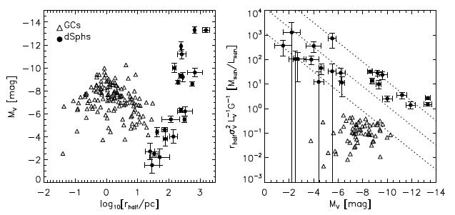 |
Figure 13. Left: Luminosity versus size (updated from Belokurov et al. 2007, Gilmore et al. 2007, Martin et al. 2008), for Milky Way satellites including objects classified as globular clusters (open triangles; data from Harris (1996, 2010 edition) and dwarf spheroidals (filled circles with error bars; data from compilations by Irwin & Hatzidimitriou 1995, Mateo 1998, Martin et al. 2008, Sand et al. 2011). The apparent lack of objects toward low luminosity and large size is a selection effect that reflects the surface-brightness limit of the SDSS survey (Koposov et al., 2008). Right: Dynamical mass-to-light ratio (modulo a constant scale factor) versus luminosity. Updated from Mateo et al. (1993), Mateo (1998), Simon & Geha (2007), Geha et al. (2009). Dotted lines correspond to constant masses of 105 M⊙, 106 M⊙ and 107 M⊙. |
The left-hand panel of Figure 13 plots luminosity against size, characterised by the projected halflight radius (Belokurov et al., 2007, Gilmore et al., 2007, Martin et al., 2008, Sand et al., 2011). Here one can appreciate another conclusion of Shapley's (1938b) regarding the first known dSphs: ‘The Sculptor and Fornax systems might be called greatly expanded giant clusters’. Indeed, while the luminosity distributions of dSphs and globular clusters overlap substantially, most dSphs have Rh ≳ 100 pc while most globular clusters have Rh ≲ 10 pc (Gilmore et al., 2007). 4 The region between 10 ≲ Rh / pc ≲ 100 is populated only by globular clusters with MV ≲ −4 or by dSphs with MV ≳ −4.
Current kinematic results suggest that this separation in luminosity between the smallest dSphs and the largest globular clusters is not merely an artifact of classification, but points to a fundamental structural difference. The right-hand panel of Figure 13 plots the product Rh σ2 / (LV G) (dimensionally a mass-to-light ratio) against luminosity. In the region of overlapping size, the less luminous objects tend to have larger velocity dispersions, amplifying the separation in luminosity such the smallest, faintest dSphs have the largest dynamical mass-to-light ratios of any known galaxies (Kleyna et al., 2005, Muñoz et al., 2006, Martin et al., 2007, Simon & Geha, 2007, Geha et al., 2009, Simon et al., 2011). 5 Furthermore, the ultrafaint dSphs extend a relation under which less luminous dSphs have larger M / LV (Mateo et al., 1993, Mateo, 1998, Section 5). The discontinuity in dynamical M / LV between dSphs and globular clusters seems to mark a boundary between objects with dark matter and those without.
1 As Figure 1 and the terms themselves suggest, the distinction between ‘classical’ and ‘ultrafaint’ dSphs involves a mixture of intrinsic luminosity with sequence of discovery. Here this distinction (which is meaningless in the sense that members of both classes trace smooth scaling relationships involving luminosity, size, metallicity and stellar kinematics) is preserved only because observational studies of these objects — for both practical and accidental reasons — tend to be separable along the same lines. Following common practice, dSphs known before SDSS (Carina, Draco, Fornax, Leo I, Leo II, Sculptor, Sextans, Ursa Minor) are referred to as ‘classical’, and the rest as ‘ultrafaint’. Back.
2 In fact RK is usually referred to as a ‘tidal’ radius and denoted rt. The adopted nomenclature and notation avoid confusion with the tidal radius defined in Equation 4. Back.
3 Aaronson added to the final article proof a measurement of −285.6 ± 1.1 km s−1 for a fourth, non-carbon star, further supporting a large dispersion. Back.
4 M31 hosts several ‘extended’ globular clusters with halflight radii as large as several tens of pc (e.g., Huxor et al., 2005), but no similar population within the Milky Way has yet been discovered. Back.
5 Some ambiguity regarding the masses of the smallest, faintest dSphs results from the convergence of three relevant quantities — the typical velocity measurement error, the measured velocity dispersions, and the potential contribution to the measured dispersions from binary orbital motions — on the same value, ∼ 3−4 km s−1 (Simon & Geha, 2007, Martin et al., 2007, McConnachie & Côté, 2010, Simon et al., 2011, Koposov et al., 2011b). For some faint dSphs the most compelling evidence for large amounts of dark matter comes from stellar-atmospheric chemistry rather than kinematics. The faintest objects classified as dSphs tend to have metallicity dispersions (σ[Fe/H] ≳ 0.4 dex, Geha et al. 2009, Norris et al. 2010, Kirby et al. 2011, Willman et al. 2011) that are indicative of prolonged and perhaps multiple episodes of star formation, thereby requiring gravitational potentials sufficiently deep to retain interstellar media despite pressures generated by stellar feedback. An adequate discussion of the relationships between dSph kinematics and stellar chemistry is beyond the scope of the present work; Tolstoy et al. (2009) provide an excellent, recent review. Back.