


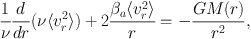
For a collisionless stellar system in dynamic equilibrium, the
gravitational potential, Φ, relates to the phase-space
distribution of stellar tracers
7,
f( ,
,
 ,
t), via the collisionless Boltzmann Equation (Equation 4-13c of
Binney & Tremaine
(2008)):
,
t), via the collisionless Boltzmann Equation (Equation 4-13c of
Binney & Tremaine
(2008)):
 |
(5) |
Current instrumentation resolves the internal distributions of neither distance nor proper motions for dSph stars. The structural and kinematic observations described in Section 2 provide information only about the projections of phase space distributions along lines of sight, limiting knowledge about f and hence also about Φ. Therefore all efforts to translate existing data sets into constraints on Φ involve simplifying assumptions. Along with dynamic equilibrium, common assumptions include spherical symmetry and particular functional forms for the distribution function and/or the gravitational potential. The most useful analyses identify the least restrictive assumptions that are appropriate for a given data set. Modern structural/kinematic data contain information that is sufficient to place reasonably robust constraints not only on the amount of dSph mass, but in some cases also on its spatial distribution.
4.1.1. ‘Mass Follows Light’ Models
A common method for analysing dSph kinematics employs the following assumptions:
1. dynamic equilibrium;
2. spherical symmetry;
3. isotropy of the velocity distribution, such that ⟨ vr2⟩ ; = ⟨ vθ2⟩ = ⟨ vφ2⟩;
4. a single stellar component;
5. the mass density profile, ρ(r), is proportional to the luminous density profile, ν(r) (i.e., M / L is constant, or ‘mass follows light’).
Historically, assumption (5) has been adopted when the velocity dispersion profile σ(R) is unavailable. Examples include early analyses of classical dSphs (Mateo, 1998, and references therein) and initial analyses of ultrafaint dSphs (e.g., Kleyna et al., 2005, Muñoz et al., 2006, Martin et al., 2007, Simon & Geha, 2007). Under this assumption, the steeply falling outer surface brightness profiles of dSphs (Section 2.2.1 and Figure 2) motivate the use of dynamical models that allow for truncation by external tides (e.g., Michie, 1963, King, 1966). Consider, for example, the model of King (1966, see also Chapter 4 of Binney & Tremaine 2008), in which the distribution function depends only on energy:
 |
(6) |
The relative potential, Ψ ≡ Φ0 − Φ, is defined such that є ≡ Ψ − 1/2 v2 ≥ 0 at radii r ≤ RK. Given the assumption that mass follows light, this model is fully specified by dimensionless parameter Ψ(0) / vs2 (or equivalently, RK / Rc), the core radius Rc and one of either the central velocity dispersion σ0 or central mass density ρ0, which are all related by Rc2 = 9σ02 / (4π Gρ0).
Illingworth (1976) shows that under assumptions (1)-(5) and a distribution function of the form specified by Equation 6, the total mass is given by
 |
(7) |
where parameter η is determined by concentration c ≡ log10[RK / Rc]. Following Mateo (1998), many authors adopt η ≈ 8, which is appropriate for the low concentrations characteristic of classical dSphs but is not well-constrained for the faintest dSphs.
More generally, Richstone & Tremaine (1986) show that for ‘almost any’ spherical, isotropic system with constant mass-to-light ratio and centrally cored luminosity profile, the dynamical mass-to-light ratio is approximately
 |
(8) |
where the half-brightness radius is defined by Σ(Rhb) = 1/2 Σ(0) and is often similar (within ∼ 25%) to Rc. Figure 17 plots dynamical mass-to-light ratios calculated from Equation 8 against dSph luminosity. Masses obtained for the Milky Way's eight classical dSphs are all Mtot ∼ 107 M⊙ (Mateo, 1998). For the ultrafaints, masses range from 105 ≲ Mtot / M⊙ ≲ 107 (Martin et al., 2007, Simon & Geha, 2007). Dynamical mass-to-light ratios increase monotonically with decreasing luminosity, ranging from 10 ≲ M / LV / [M / LV]⊙ ≲ 1000.
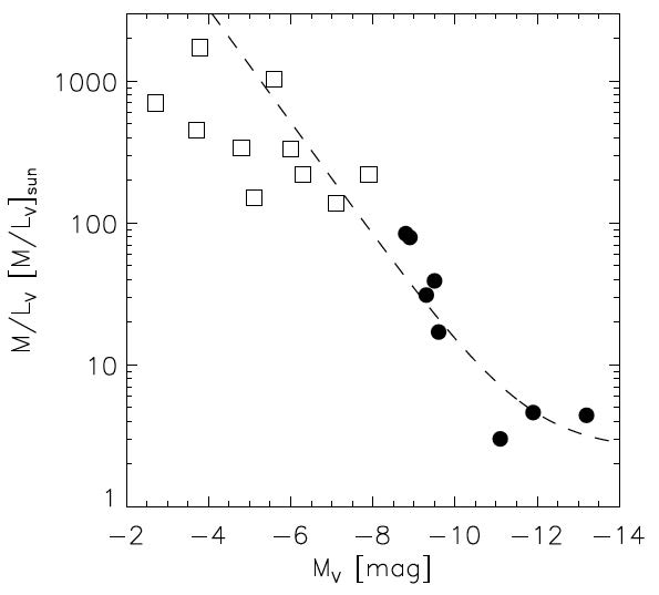 |
Figure 17. Dynamical mass-to-light ratio, derived from mass-follows-light models (Section 4.1.1), versus luminosity. Data for the Milky Way's ‘classical’ dSphs (filled circles) are from the review of Mateo (1998). Data for the ‘ultrafaint’ dSphs (open squares) are from Keck/DEIMOS observations by Simon & Geha (2007) and Martin et al. (2007). The dotted line corresponds to [M / LV / [M / LV]⊙] = 2.5 + 107 / (L / LV,⊙) (Section 5). |
4.1.2. Does Mass Follow Light?
When available, empirical velocity dispersion profiles provide simple tests of the assumptions listed above. Dashed lines in Figure 12 display best-fitting King (1966, Equation 6) models constructed under assumptions (1)-(5), fit to the surface brightness profiles of Irwin & Hatzidimitriou (1995, Figure 2), and normalised to fit the central velocity dispersions. For all of the Milky Way's classical dSphs, the central velocity dispersions imply large mass-to-light ratios M / LV ≳ 10 [M / LV]⊙, as plotted in Figure 17. However, the mass-follows-light models underpredict the observed velocity dispersions at large radii, which tend to remain approximately constant out to the outermost measured points.
These discrepancies between empirical velocity dispersion profiles and mass-follows-light models in Figure 12 imply that at least one of assumptions (1)-(5) is invalid. In fact all are invalid at some level. However, various studies indicate that it is unlikely any one of assumptions (1)-(4) alone can be the problem. For example:
1. Simulations by Read et al. (2006a) suggest that tidal disruption (a violation of the equilibrium assumption) is more likely to generate rising velocity dispersion profiles rather than the flat profiles observed for real dSphs.
2. Axisymmetric models of Fornax considered by Jardel & Gebhardt (2011, see Section 4.2.2) favor dark matter halos that, while violating the assumption of spherical symmetry, extend well beyond the luminous component and therefore also invalidate the mass-follows-light assumption.
3. Evans, An & Walker (2009) derive analytically an expression for the anisotropy profile, βa(r) ≡ 1 − ⟨ vθ2⟩ / ⟨ vr2⟩ in terms of surface brightness and velocity dispersion profiles. If mass follows light, then the flat empirical velocity dispersion profiles tend to imply unphysical values βa > 1.
4. While recent observations indicate that some dSphs contain at least two distinct stellar sub-populations (Sections 2.2.4 and 4.2.2), scale radii of the individual sub-populations are sufficiently well constrained (e.g., Battaglia et al., 2006, Battaglia et al., 2008) that superpositions of two mass-follows-light models continue to underpredict the observed velocity dispersions at large radii. Indeed Battaglia et al. (2008) find that the flat velocity dispersion profile they measure for Sculptor's more spatially extended subpopulation continues to imply an even more extended dark matter halo.
Models that allow for sufficiently extended dark matter halos (violating assumption (5) while retaining assumptions (1)-(4)) can provide good fits to surface brightness and velocity dispersion profiles simultaneously (e.g., Pryor & Kormendy, 1990, Wilkinson et al., 2002). On these grounds, the empirical profiles shown in Figures 2 and 12 provide the strongest available evidence that dSphs have dominant dark matter halos that extend beyond luminous regions.
Some scenarios for dSph formation and evolution — particularly the tidal stirring mechanism of Mayer et al. (2001a, b, Section 3.2) and the tidal disruption simulations of Muñoz et al. (2008) — tend to produce configurations in which mass approximately follows light. The results discussed above seem to rule out this configuration. However, Łokas (2009) finds reasonable agreement with mass-follows-light models in Carina, Fornax, Sculptor and Sextans after trimming velocity samples in order to remove member stars classified by an iterative mass estimator (Klimentowski et al., 2007) as unbound. This result rests in part on a circular argument, as the adopted mass estimator (Heisler et al., 1985) is based on the virial theorem, which itself assumes mass follows light. However, the same charge of circularity can be brought against the standard kinematic analysis, in which the inclusion of stars at large radius in the kinematic analysis implicitly assumes they are bound by a sufficiently extended dark matter halo. Thus conclusions regarding the extended structure of dSph dark matter halos are generally sensitive to the assumptions employed when determining which stars to consider or reject in kinematic analyses. More secure is the conclusion that dark matter dominates dSph potentials: even mass-follows-light models require central mass-to-light ratios M / LV ≳10 [M / LV]⊙ in order to fit the central velocity dispersions of dSphs (Muñoz et al., 2008, Łokas, 2009, and Figure 12).
The methods for mass estimation described in the previous section either
employ directly or are derived from specific distribution functions
f(,
) that correspond
to physical dynamical models restricted by particular
assumptions. Integration of Equation 5 over velocity space provides an
alternative starting point in the form of the Jeans equations (see
Binney & Tremaine,
2008).
With spherical symmetry one obtains
 |
(9) |
where ν(r), ⟨
vr2⟩ (r), and
βa(r) ≡ 1 − ⟨
vθ2⟩ / ⟨
vr2⟩ describe the 3-dimensional
density, radial velocity dispersion, and orbital anisotropy,
respectively, of the (stellar) tracer component. The mass profile,
M(r), includes contributions from any dark matter
halo. While there is no requirement that mass follow light, there is
also no guarantee that a given solution to Equation 9 — even one
that fits the data — corresponds to a physical dynamical model
(i.e., one for which
f(,
) is non-negative).
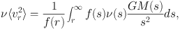
Equation 9 has general solution (van der Marel, 1994, Mamon & Łokas, 2005)
 |
(10) |
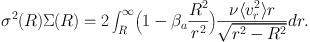
where f(r) = 2f(r1) exp ∫r1r βa(s) s−1 ds. Projecting along the line of sight, the mass profile relates to observable profiles, the projected stellar density, Σ(R) (Figure 2), and velocity dispersion, σ(R) (Figure 12), according to (Binney & Tremaine, 2008)
 |
(11) |
Equation 11 forms the basis for many methods of mass estimation, including parametric (e.g., Strigari et al., 2006, 2008a, Strigari, 2010, Koch et al., 2007b, a, Battaglia et al., 2008, Walker et al., 2007b, b, Martinez et al., 2011) and nonparametric (e.g. Wang et al., 2005) techniques as well as algebraic inversion (e.g., Wilkinson et al., 2004, Gilmore et al., 2007).
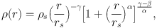
All methods based on Equation 11 are limited fundamentally by a degeneracy between the function of interest, M(r), and the anisotropy profile, βa(r), which is poorly constrained by velocity data confined to the line of sight. 8 Consideration of a common parametric method helps to illustrate this limitation. For example, it is common to assume that the the gravitational potential is dominated everywhere by a dark matter halo with mass density profile
 |
(12) |
i.e., the generalisation by Zhao (1996) of the Hernquist (1990) profile. Equation 12 provides a flexible halo model in the form of a split power-law, with free parameter α controlling the transition from index −γ at small radii (r ≪ rs) to a value of −β at large radii (r ≫ rs).
From spherical symmetry, the density profile specifies the mass profile via
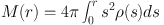 |
(13) |
and the surface brightness profile specifies the (deprojected) stellar density profile via
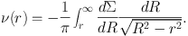 |
(14) |
Given values for free parameters ρs, rs, α, β, γ and an assumption about the otherwise unconstrained anisotropy profile 9, Equation 11 specifies a product Σ(R) σ2(R) that can then be compared with observations.
Using Sculptor as an example, Figure 18 demonstrates the degeneracy that is inherent in the standard Jeans analysis. Overplotted on Sculptor's empirical velocity dispersion profile are best-fitting models obtained under specific assumptions either about the inner slope of the mass-density profile (γ = 0 or γ = 1), or about the amount of velocity anisotropy (βa = −0.5, βa = 0 or βa = +0.3). Despite corresponding to a wide range of total masses and mass distributions (bottom panels of Figure 18), all of these models can provide equivalent fits to the structural and kinematic data.
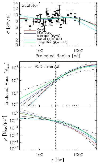 |
Figure 18. Degeneracy in the Jeans analysis of dSph mass profiles (Section 4.1.3). In the top panel, overplotted on Sculptor's empirical velocity dispersion profile are best-fitting cored (γ = 0 in the notation of Equation 12) and cusped (γ = 1) density profiles, as well as models that assume isotropic (βa = 0), radially anisotropic (βa = +0.3) and tangentially anisotropic (βa = −0.5) velocity distributions. All of these models provide equivalent fits to the data. The bottom two panels plot mass and density profiles corresponding to each model. Dotted curves indicate 95% confidence intervals, as determined from a Jeans/MCMC analysis that assumes constant anisotropy and lets the unspecified parameters in Equation 12 vary freely (Section 4.1.3). The vertical dotted line indicates Sculptor's projected halflight radius. |
While the Jeans analysis provides useful constraints on none of the halo parameters included in Equation 12, it does imply a model-independent constraint on a basic dynamical quantity. All models that fit the velocity dispersion profile give approximately the same value for the enclosed mass near the halflight radius (middle panel of Figure 18), indicating that this quantity is well determined by the available data. Indeed, formal confidence intervals derived from Markov-Chain Monte Carlo scans of the full parameter space (e.g., Strigari et al., 2007a, Strigari, 2010, Walker et al., 2009b, Wolf et al., 2010, Martinez et al., 2011) show a characteristic ‘pinch’ near the halflight radius (Figure 18).
Equivalent constraints on the enclosed mass at the halflight radius can be obtained more simply by solving Equation 9 under the assumptions that βa = 0 and σ(R) = constant. For a Plummer surface brightness profile (Equation 3), one obtains (Walker et al., 2009b)
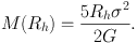 |
(15) |
Wolf et al. (2010) show analytically that for various surface brightness and anisotropy profiles, the tightest constraint on the mass profile (provided that the velocity dispersion profile is sufficiently flat) can be approximated by
 |
(16) |
where r3 is the radius at which dlnν / dlnr = −3. For most commonly-adopted surface brightness profiles, this radius is close to the deprojected halflight radius (i.e., the radius of the sphere containing half of the stars), which typically exceeds the projected halflight radius by a factor of ∼ 4/3. Insofar as the assumption of flat velocity dispersion profiles (and the usual assumptions of dynamic equilibrium and spherical symmetry) holds, these simple mass estimators can be applied even to the relatively sparse kinematic data available for ultrafaint satellites. Walker et al. (2009b, see erratum for updated values) and Wolf et al. (2010) tabulate masses obtained from Equations 15 and 16, respectively, for ∼ 2 dozen Local Group dSphs.
The equivalence of such seemingly crude estimates to constraints from Jeans/MCMC explorations of parameter space follows from a combination of facts: 1) Equation 9 deals only with velocity moments of the phase space distribution function and not with the distribution function itself; 2) confinement of empirical velocity distributions to the line-of-sight component yields little information about βa; 3) therefore the flat velocity dispersion profiles of dSphs effectively reduce the available kinematic information to just two numbers, σ and the scale radius that characterises the adopted surface brightness profile. The information extracted from the Jeans analysis naturally amounts to a simple combination of these two numbers.
Some cosmological and particle physics models make specific predictions about how dark matter is distributed within individual halos (Section 6). Insofar as dSphs represent the structures most dominated by dark matter and least affected by the presence of baryons, their internal dynamical properties provide the most straightforward tests of such predictions. Section 4.1.3 demonstrates that so long as dSphs have flat velocity dispersion profiles, the standard Jeans analysis constrains only one number, characterising the amount but not the distribution of dark matter. However, the restrictive assumptions employed in the standard Jeans analysis overlook structure that is present in the data available for many dSphs (Section 2.2.4). Recent analyses that are devised to exploit more fully the available empirical information have been able to place useful constraints not only on the amount, but also on the distribution of dark matter within individual dSphs.
The presence of stellar substructure within dSphs can provide extra leverage not easily exploited in the context of equilibrium dynamical models. For example, it has long been known that Ursa Minor's stellar component is ‘lumpy’ (Hodge, 1964b, Olszewski & Aaronson, 1985, Irwin & Hatzidimitriou, 1995, Palma et al., 2003, Section 2.2.4). While Ursa Minor has a velocity dispersion of σ ∼ 10 km s−1, Kleyna et al. (2003) find that a secondary peak in Ursa Minor's stellar density field, offest by ∼ 20′ (∼ 400 pc) from the nominal center, exhibits a cold dispersion of ≲ 1 km s−1. Interpreting this feature as a loosely bound star cluster captured by Ursa Minor, Kleyna et al. (2003) perform N-body simulations to examine how its stability depends on the external gravitational potential (assumed to be dominated by dark matter) of Ursa Minor. Whereas simulated clusters remain intact for a Hubble time when the host potential has a central ‘core’ with constant density (γ = 0 in the notation of Equation 12) on scales larger than the orbital radius, they disrupt on timescales of ≲ 1 Gyr when the host potential has a centrally divergent, or ‘cusped’ density profile (γ > 1/2). Therefore, if the observed clump indeed corresponds to a star cluster free of its own dark matter component, then its survival provides indirect evidence that the dark matter density of Ursa Minor is constant over the central few-hundred pc.
Substructure in the form of Fornax's five globular clusters provides another example of indirect evidence for a cored dSph potential. Four of these clusters are projected near (within a factor of ∼ 2) Fornax's halflight radius (Rh ∼ 670 pc; Irwin & Hatzidimitriou (1995)). Hernandez & Gilmore (1998) show analytically that the rate at which the orbits of such clusters decay due to dynamical friction depends on the underlying dSph potential. Subsequent numerical simulations by Sánchez-Salcedo et al. (2006) and Goerdt et al. (2006) demonstrate that in a cusped potential, dynamical friction would require only a few Gyr to bring the clusters from their present positions (assuming the projected distances from Fornax's center are not much smaller than the true distances) all the way to Fornax's center. On the other hand, in a cored potential dynamical friction would bring the clusters only as close as the core radius, where the harmonic potential inhibits further decay. Thus these considerations provide indirect evidence for a core of constant density over the central few-hundred pc in Fornax. Further simulations by Goerdt et al. (2010) and Cole et al. (2011) suggest that the transfer of angular momentum from a sinking cluster to the central dark matter is capable of transforming an originally cusped into a cored potential, a possibility that might be relevant for the interpretation of evidence for cored dark matter halos in some dSphs (Section 6.1).
4.2.2. Constraints from Models
Several groups have recently developed dynamical and/or kinematic models that exploit structure that is present in dSph data but is not considered in the Jeans analyses discussed in Section 4.1.3. For example, the discoveries of two chemo-dynamically independent stellar sub-populations in Sculptor (Tolstoy et al., 2004, Section 2.2.4), Fornax (Battaglia et al., 2006) and Sextans (Battaglia et al., 2011) enable analyses of two tracer components in the same potential. After imposing a metallicity cutoff to separate Sculptor's two sub-populations, Battaglia et al. (2008) find that cored rather than cusped potentials provide better simultaneous fits in a Jeans analysis (Section 4.1.3) of the two sets of surface brightness and velocity dispersion profiles. Using the same empirical profiles for Sculptor, Amorisco & Evans (2012) confirm this result by modelling both sub-populations with anisotropic King-Michie (King, 1962, Michie, 1963, King, 1966) distribution functions. These dynamical models again favor cored (γ = 0) rather than cusped (γ = 1) potentials, with a likelihood ratio sufficient to reject the hypothesis of cusped potentials with confidence ≳ 99%.
Jardel & Gebhardt (2011) take a different approach, constructing axisymmetric three-integral Schwarzschild (1979) models for both cored and cusped potentials that also allow for a central black hole. For a given potential, libraries of stellar orbits are calculated and each orbit receives a weight based on fits to the observed distribution of velocities within discretely binned radii. Notice that while the Jeans analysis is sensitive only to the variance of the velocity distribution in a given bin, the Schwarzschild method is sensitive to the shape of the distribution. Jardel & Gebhardt (2011) find that their models constructed from cored potentials fit Fornax's velocity data significantly better than those constructed from cusped potentials. Within the context of their adopted models, they also place an upper limit of ≲ 3.2 × 10⁴ M⊙ on the mass of any central black hole. Breddels et al. (2012) independently develop Schwarzschild models for Sculptor, concluding that the available data rule out steep cusps (γ ≳ 1.5) but are consistent with slopes in the range 0 ≲ γ ≲ 1. 10
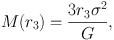
Walker & Peñarrubia (2011) introduce a method for measuring the slopes of dSph mass profiles directly from spectroscopic data and without adopting a dark matter halo model. For a given dSph, Walker & Peñarrubia (2011) use measurements of stellar positions, velocities and spectral indices to estimate halflight radii and velocity dispersions for as many as two chemo-dynamically independent stellar sub-populations. Detections of two distinct sub-populations with different sizes provide mass estimates M(Rh) ∝ Rh σ2 (e.g., Equation 15) at two different radii in the same mass profile, immediately specifying a slope. For Fornax and Sculptor, this method yields slopes of Γ ≡ Δ logM / Δ logr = 2.61−0.37+0.43 and Γ = 2.95−0.390.51, respectively, on scales defined by values ∼ 0.2 ≲ Rh / kpc ≲ 1 estimated for the halflight radii. These slopes are consistent with cored (γ = 0) potentials, for which Γ ≤ 3 at all radii, but incompatible with cusped (γ ≳ 1) potentials, for which Γ ≤ 2 (Figure 19).
 |
Figure 19. Empirical constraints on the slopes of mass profiles in Fornax and Sculptor, based on estimates of M(rh) for each of two chemo-dynamically independent stellar sub-populations in each galaxy (Section 4.2.3, Walker & Peñarrubia 2011, reproduced by permission of the American Astronomical Society). Points in the left two panels indicate constraints on the two halflight radii and masses enclosed therein, with lines indicating the maximum slopes allowed for cored (γ = 0 in the notation of Equation 12; Γ ≡ Δ logM / Δ logr ≤ 3) and cusped (γ = 1, Γ≤ 2) overplotted. The right-hand panel indicates posterior probability distributions for the slope in each galaxy. The data rule out the cuspy (γ ≳ 1, Γ ≤ 2) profiles that characterise the cold dark matter halos produced in cosmological simulations (e.g., Navarro, Frenk & White, 1997) with significance ≳ 96% and ≳ 99% in Fornax and Sculptor, respectively. |
7 The distribution function is defined
such that
f(,
, t)
d3 d3
specifies the number of stars inside the volume of phase space
d3
d3
centered on (,
) at time t.
Back.
d3
specifies the number of stars inside the volume of phase space
d3
d3
centered on (,
) at time t.
Back.
8 Łokas et al. (2005) develop a Jeans analysis that uses higher-order velocity moments (e.g., ⟨v4⟩) in order to reduce degeneracy between anisotropy (assumed to be constant) and total mass (effectively normalising a cusped mass profile that is assumed to have γ = 1 in the notation of Equation 12). Back.
9 Typical assumptions about anisotropy range in simplicity from βa = 0 or βa = constant to βa(r) = (β∞ − β0) r2 / (rβ2 + r2) + β0 (e.g., Strigari, 2010), introducing as many as three new free parameters. Back.
10 Chanamé et al. (2008) have formulated a Schwarzschild method that operates on discrete velocity measurements, avoiding the binning procedure altogether. Efforts to apply this and other discrete Schwarzschild methods to dSph data are underway. As these and other methods for analysing the shapes of dSph velocity distributions continue to develop, it will be beneficial and perhaps necessary to allow for contributions from multiple stellar populations. Failure to consider distinct populations can generate spurious conclusions regarding orbital structure. To see why this is so, consider that the superposition of two Gaussian distributions need not be Gaussian. Back.