


8.1. The Cosmic Star Formation History
One of the major goals of the study of galaxy formation is to achieve
an observational determination and a theoretical understanding of the
cosmic star formation history. By now, this history has been sketched
out to a redshift z ~ 4 (see, e.g., the compilation of
Blain et al. 1999a).
This is based on a large number of observations in
different wavebands. These include various
ultraviolet/optical/near-infrared observations
(Madau et al. 1996;
Gallego et al. 1996;
Lilly et al. 1996;
Connolly et al. 1997;
Treyer et al. 1998;
Tresse & Maddox 1998;
Pettini et al. 1998a,
b;
Cowie, Songaila &
Barger 1999;
Gronwall 1999;
Glazebrook et al. 1999;
Yan et al. 1999;
Flores et al. 1999;
Steidel et al. 1999).
At the shortest wavelengths, the extinction correction is likely to be
large (a factor of ~ 5) and is still highly uncertain. At longer
wavelengths, the star formation history has been reconstructed from
submillimeter observations
(Blain et al. 1999b;
Hughes et al. 1998)
and radio observations
(Cram 1998).
In the submillimeter regime, a
major uncertainty results from the fact that only a minor portion of
the total far infrared emission of galaxies comes out in the observed
bands, and so in order to estimate the star formation rate it is
necessary to assume a spectrum based, e.g., on a model of the dust
emission (see the discussion in
Chapman et al. 2000).
In general, estimates of the star formation rate (hereafter SFR) apply
locally-calibrated correlations between emission in particular lines
or wavebands and the total SFR. It is often not possible to check
these correlations directly on high-redshift populations, and together
with the other uncertainties (extinction and incompleteness) this
means that current knowledge of the star formation history must be
considered to be a qualitative sketch only. Despite the relatively
early state of observations, a wealth of new observatories in all
wavelength regions promise to greatly advance the field. In
particular, NGST will be able to detect galaxies and hence
determine the star formation history out to z
 10.
10.
Hierarchical models have been used in many papers to match observations on
star formation at z
 4 (see, e.g.
Baugh et al. 1998;
Kauffmann & Charlot
1998;
Somerville & Primack
1998,
and references therein). In
this section we focus on theoretical predictions for the cosmic star
formation rate at higher redshifts. The reheating of the IGM during
reionization suppressed star formation inside the smallest halos
(Section 6.5). Reionization is therefore
predicted to cause a drop in
the cosmic SFR. This drop is accompanied by a dramatic fall in the
number counts of faint galaxies.
Barkana & Loeb (2000b)
argued that a detection of this fall in the faint luminosity function
could be used to identify the reionization redshift observationally.
4 (see, e.g.
Baugh et al. 1998;
Kauffmann & Charlot
1998;
Somerville & Primack
1998,
and references therein). In
this section we focus on theoretical predictions for the cosmic star
formation rate at higher redshifts. The reheating of the IGM during
reionization suppressed star formation inside the smallest halos
(Section 6.5). Reionization is therefore
predicted to cause a drop in
the cosmic SFR. This drop is accompanied by a dramatic fall in the
number counts of faint galaxies.
Barkana & Loeb (2000b)
argued that a detection of this fall in the faint luminosity function
could be used to identify the reionization redshift observationally.
A model for the SFR can be constructed based on the extended Press-Schechter theory. The starting point is the abundance of dark matter halos, obtained using the Press-Schechter model. The abundance of halos evolves with redshift as each halo gains mass through mergers with other halos. If dp[M1, t1 -> M, t] is the probability that a halo of mass M1 at time t1 will have merged to form a halo of mass between M and M + dM at time t > t1, then in the limit where t1 tends to t we obtain an instantaneous merger rate d2p[M1 -> M, t] / (dM dt). This quantity was evaluated by Lacey & Cole [1993, their equation (2.18)], and it is the basis for modeling the rate of galaxy formation.
Once a dark matter halo has collapsed and virialized, the two requirements for forming new stars are gas infall and cooling. We assume that by the time of reionization, photo-dissociation of molecular hydrogen (see Section 3.3) has left only atomic transitions as an avenue for efficient cooling. Before reionization, therefore, galaxies can form in halos down to a circular velocity of Vc ~ 17 km s-1, where this limit is set by cooling. On the other hand, when a volume of the IGM is ionized by stars or quasars, the gas is heated and the increased pressure suppresses gas infall into halos with a circular velocity below Vc ~ 80 kmI>s-1, halting infall below Vc ~ 30 km s-1 (Section 6.5). Since the suppression acts only in regions that have been heated, the reionization feedback on galaxy formation depends on the fraction of the IGM which is ionized at each redshift. In order to include a gradual reionization in the model, we take the simulations of Gnedin (2000a) as a guide for the redshift interval of reionization.
In general, new star formation in a given galaxy can occur either from
primordial gas or from recycled gas which has already undergone a previous
burst of star formation. The former occurs when a massive halo accretes gas
from the IGM or from a halo which is too small to have formed stars. The
latter occurs when two halos, in which a fraction of the gas has already
turned to stars, merge and trigger star formation in the remaining
gas. Numerical simulations of starbursts in interacting z = 0 galaxies
(e.g.,
Mihos & Hernquist
1994;
1996)
found that a merger triggers
significant star formation in a halo even if it merges with a much less
massive partner. Preliminary results (Somerville 2000, private
communication) from simulations of mergers at z ~ 3 find that they
remain effective at triggering star formation even when the initial disks
are dominated by gas. Regardless of the mechanism, we assume that feedback
limits the star formation efficiency, so that only a fraction
 of
the gas is turned into stars.
of
the gas is turned into stars.
Given the SFR and the total number of stars in a halo of mass M, the
luminosity and spectrum can be derived from an assumed stellar initial
mass function. We assume an initial mass function which is similar to
the one measured locally. If n(M) is the total number of
stars with masses less than M, then the stellar initial mass function,
normalized to a total mass of
1M , is
(Scalo 1998)
, is
(Scalo 1998)
| (97) |
where M1 = M /
M. We assume
a metallicity Z = 0.001, and use the stellar population model
results of
Leitherer et al. (1999)
(6) .
We also include a Ly cutoff
in the spectrum due to absorption by the
dense Ly forest. We do not,
however, include dust extinction,
which could be significant in some individual galaxies despite the low
mean metallicity expected at high redshift.
cutoff
in the spectrum due to absorption by the
dense Ly forest. We do not,
however, include dust extinction,
which could be significant in some individual galaxies despite the low
mean metallicity expected at high redshift.
Much of the star formation at high redshift is expected to occur in
low mass, faint galaxies, and even NGST may only detect a fraction of
the total SFR. A realistic estimate of this fraction must include the
finite resolution of the instrument as well as its detection limit for
faint sources
(Barkana & Loeb
2000a).
We characterize the
instrument's resolution by a minimum circular aperture of angular
diameter  a. We
describe the sensitivity of NGST by
F
a. We
describe the sensitivity of NGST by
F ps,
the minimum spectral flux
(7) ,
averaged over wavelengths
0.6-3.5µm, required to detect a point source (i.e., a source which
is much smaller than
a). For an
extended source of diameter
s >>
a, we assume that
the signal-to-noise ratio can
be improved by using a larger aperture, with diameter
s. The
noise amplitude scales as the square root of the number of noise (sky)
photons, or the square root of the corresponding sky area. Thus, the
total flux needed for detection of an extended source at a given
signal-to-noise threshold is larger than
Fps by a
factor of s /
a. We adopt a
simple interpolation
formula between the regimes of point-like and extended sources, and
assume that a source is detectable if its flux is at least
sqrt[1 + (s /
a)2]
Fps.
ps,
the minimum spectral flux
(7) ,
averaged over wavelengths
0.6-3.5µm, required to detect a point source (i.e., a source which
is much smaller than
a). For an
extended source of diameter
s >>
a, we assume that
the signal-to-noise ratio can
be improved by using a larger aperture, with diameter
s. The
noise amplitude scales as the square root of the number of noise (sky)
photons, or the square root of the corresponding sky area. Thus, the
total flux needed for detection of an extended source at a given
signal-to-noise threshold is larger than
Fps by a
factor of s /
a. We adopt a
simple interpolation
formula between the regimes of point-like and extended sources, and
assume that a source is detectable if its flux is at least
sqrt[1 + (s /
a)2]
Fps.
We combine this result with a model for the distribution of disk sizes
at each value of halo mass and redshift
(Section 5.1). We adopt a value of
Fps =
0.25 nJy
(8) , assuming a deep 300-hour
integration on an 8-meter NGST and a spectral resolution of
10:1. This resolution should suffice for a ~ 10% redshift
measurement, based on the Ly
cutoff. We also choose the aperture diameter to be
a = 0".06, close
to the expected NGST resolution at 2µm.
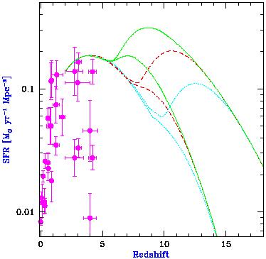
Figure 29 shows our predictions for the star formation
history of the universe, adopted from Figure 1 of
Barkana & Loeb (2000b)
with slight modifications (in the initial mass function and
the values of the cosmological parameters). Letting
zreion denote the
redshift at the end of overlap, we show the SFR for
zreion = 6 (solid
curves), zreion = 8 (dashed curves), and
zreion = 10 (dotted curves). In
each pair of curves, the upper one is the total SFR, and the lower one
is the fraction detectable with NGST. The curves assume a star
formation efficiency
= 10% and an IGM temperature
TIGM = 2 × 10⁴ K. Although
photoionization directly suppresses new gas
infall after reionization, it does not immediately affect mergers
which continue to trigger star formation in gas which had cooled prior
to reionization. Thus, the overall suppression is dominated by the
effect on star formation in primordial (unprocessed) gas. The
contribution from merger-induced star formation is comparable to that
from primordial gas at
z < zreion, and it is smaller at
z > zreion. However,
the recycled gas contribution to the detectable SFR is dominant
at the highest redshifts, since the brightest, highest mass halos form
in mergers of halos which themselves already contain stars. Thus, even
though most stars at
z > zreion form out of primordial,
zero-metallicity gas, a majority of stars in detectable galaxies may
form out of the small gas fraction that has already been enriched by
the first generation of stars.
|
Figure 29. Redshift evolution of the SFR (in
M |
Points with error bars in Figure 29 are observational
estimates of the cosmic SFR per comoving volume at various redshifts
(as compiled by
Blain et al. 1999a).
We choose = 10%
to obtain
a rough agreement between the models and these observations at z
~ 3-4. An efficiency of order this value is also suggested by
observations of the metallicity of the
Ly forest at z = 3
(Haiman & Loeb
1999b).
The SFR curves are roughly proportional to the
value of .
Note that in reality
may depend on the halo
mass, since the effect of supernova feedback may be more pronounced in
small galaxies (Section 7).
Figure 29 shows a sharp
rise in the total SFR at redshifts higher than
zreion. Although only a
fraction of the total SFR can be detected with NGST, the
detectable SFR displays a definite signature of the reionization
redshift. However, current observations at lower redshifts demonstrate
the observational difficulty in measuring the SFR directly. The
redshift evolution of the faint luminosity function provides a
clearer, more direct observational signature. We discuss this topic next.
As shown in the previous section, the cosmic star formation history should display a signature of the reionization redshift. Much of the increase in the star formation rate beyond the reionization redshift is due to star formation occurring in very small, and thus faint, galaxies. This evolution in the faint luminosity function constitutes the clearest observational signature of the suppression of star formation after reionization.
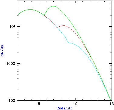
Figure 30 shows the predicted redshift distribution in
 CDM (with parameters given
at the end of Section 1) of
galaxies observed with NGST. The plotted quantity is dN /
dz,
where N is the number of galaxies per NGST field of view
(4' × 4'). The model predictions are shown for a
reionization redshift zreion = 6 (solid curve),
zreion = 8 (dashed curve),
and zreion = 10 (dotted curve), with a star formation
efficiency
= 10%. All curves
assume a point-source detection limit of 0.25
nJy. This plot is updated from Figure 7 of
Barkana & Loeb
(2000a)
in that redshifts above zreion are included.
CDM (with parameters given
at the end of Section 1) of
galaxies observed with NGST. The plotted quantity is dN /
dz,
where N is the number of galaxies per NGST field of view
(4' × 4'). The model predictions are shown for a
reionization redshift zreion = 6 (solid curve),
zreion = 8 (dashed curve),
and zreion = 10 (dotted curve), with a star formation
efficiency
= 10%. All curves
assume a point-source detection limit of 0.25
nJy. This plot is updated from Figure 7 of
Barkana & Loeb
(2000a)
in that redshifts above zreion are included.
|
Figure 30.
Predicted redshift distribution of galaxies observed with
NGST, adopted and modified from Figure 7 of
Barkana & Loeb
(2000a).
The distribution in the
|
Clearly, thousands of galaxies are expected to be found at high
redshift. This will allow a determination of the luminosity function
at many redshift intervals, and thus a measurement of its evolution.
As the redshift is increased, the luminosity function is predicted to
gradually change shape during the overlap era of reionization.
Figure 31 shows the predicted evolution of the
luminosity function for various values of
zreion. This Figure is adopted from Figure 2 of
Barkana & Loeb (2000b)
with modifications (in the initial
mass function, the values of the cosmological parameters, and the plot
layout). All curves show d2N / (dz d ln
Fps),
where N is the total number of galaxies in a single field of view of
NGST, and
Fps
is the limiting point source flux at
0.6-3.5µm for NGST. Each panel shows the result for a
reionization redshift zreion = 6 (solid curve),
zreion = 8 (dashed curve),
and zreion = 10 (dotted curve).
Figure 31 shows the luminosity
function as observed at z = 5 (upper left panel) and (proceeding
clockwise) at z = 7, z = 9, and z = 11. Although
our model assigns a
fixed luminosity to all halos of a given mass and redshift, in reality
such halos would have some dispersion in their merger histories and
thus in their luminosities. We thus include smoothing in the plotted
luminosity functions. Note the enormous increase in the number density
of faint galaxies in a pre-reionization universe. Observing this
dramatic increase toward high redshift would constitute a clear
detection of reionization and of its major effect on galaxy formation.

|
Figure 31.
Predicted luminosity function of galaxies at a fixed
redshift, adopted and modified from Figure 2 of
Barkana & Loeb
(2000b).
With |
Dynamical studies indicate that massive black holes exist in the centers of most nearby galaxies (Richstone et al. 1998; Kormendy & Ho 2000; Kormendy 2000, and references therein). This leads to the profound conclusion that black hole formation is a generic consequence of galaxy formation. The suggestion that massive black holes reside in galaxies and power quasars dates back to the sixties (Zel'dovich 1964; Salpeter 1964; Lynden Bell 1969). Efstathiou & Rees (1988) pioneered the modeling of quasars in the modern context of galaxy formation theories. The model was extended by Haehnelt & Rees (1993) who added more details concerning the black hole formation efficiency and lightcurve. Haiman & Loeb (1998) and Haehnelt, Natarajan, & Rees (1998) extrapolated the model to high redshifts. All of these discussions used the Press-Schechter theory to describe the abundance of galaxy halos as a function of mass and redshift. More recently, Kauffmann & Haehnelt (2000; also Haehnelt & Kauffmann 2000) embedded the description of quasars within semi-analytic modeling of galaxy formation, which uses the extended Press-Schechter formalism to describe the merger history of galaxy halos.
In general, the predicted evolution of the luminosity function of
quasars is constrained by the need to match the observed quasar
luminosity function at redshifts z
5, as well as data from the
Hubble Deep Field (HDF) on faint point-sources. Prior to
reionization, we may assume that quasars form only in galaxy halos
with a circular velocity
10 km s-1 (or equivalently a
virial temperature
104 K), for which cooling by atomic
transitions is effective. After reionization, quasars form only in
galaxies with a circular velocity
50 km
s-1, for which
substantial gas accretion from the warm (~ 104 K) IGM is
possible. The limits set by the null detection of quasars in the HDF
are consistent with the number counts of quasars which are implied by
these thresholds
(Haiman, Madau, &
Loeb 1999).
For spherical accretion of ionized gas, the bolometric luminosity emitted by a black hole has a maximum value beyond which radiation pressure prevents gas accretion. This Eddington luminosity (Eddington 1926) is derived by equating the radiative repulsive force on a free electron to the gravitational attractive force on an ion in the plasma,
| (98) |
where  T = 6.65 ×
10-25 cm2 is the Thomson
cross-section, µemp is the
average ion mass per electron, and
Mbh is the black hole mass. Since both forces scale as
r-2,
the limiting Eddington luminosity is independent of radius r in the
Newtonian regime, and for gas of primordial composition is given by,
T = 6.65 ×
10-25 cm2 is the Thomson
cross-section, µemp is the
average ion mass per electron, and
Mbh is the black hole mass. Since both forces scale as
r-2,
the limiting Eddington luminosity is independent of radius r in the
Newtonian regime, and for gas of primordial composition is given by,
| (99) |
Generically, the Eddington limit applies to within a factor of order unity also to simple accretion flows in a non-spherical geometry (Frank, King, & Raine 1992).
The total luminosity of a black hole is related to its mass accretion
rate by the radiative efficiency,
 ,
,

| (100) |
For accretion through a thin Keplerian disk onto a Schwarzschild
(non-rotating) black hole,
= 5.7%, while for a
maximally rotating Kerr black hole,
= 42%
(Shapiro & Teukolsky
1983,
p. 429). The
thin disk configuration, for which these high radiative efficiencies are
attainable, exists for Ldisk
0.5LE
(Laor & Netzer 1989).
The accretion time can be defined as
| (101) |
This time is comparable to the dynamical time inside the central kpc
of a typical galaxy,
tdyn ~ (1 kpc/100 km
s-1) = 107 yr. As long as its fuel
supply is not limited
and is constant, a
black hole radiating at the Eddington
limit will grow its mass exponentially with an e-folding time equal
to  . The fact that
is much shorter than the age of the
universe even at high redshift implies that black hole growth is
mainly limited by the feeding rate
. The fact that
is much shorter than the age of the
universe even at high redshift implies that black hole growth is
mainly limited by the feeding rate
 bh(t), or by the
total fuel reservoir, and not by the Eddington limit.
bh(t), or by the
total fuel reservoir, and not by the Eddington limit.
The ``simplest model'' for quasars involves the following three assumptions (Haiman & Loeb 1998):
Note that these assumptions relate only to the most luminous phase of
the black hole accretion process, and they may not be valid during
periods when the radiative efficiency or the mass accretion rate is
very low. Such periods are not of interest here since they do not
affect the luminosity function of bright quasars, which is the
observable we wish to predict. The first of the above assumptions is
reasonable as long as the fraction of virialized baryons in the
universe is much smaller than unity; it does not include a separate
mechanism for fueling black hole growth during mergers of
previously-formed galaxies, and thus, under this assumption, black
holes would not grow in mass once most of the baryons were virialized.
The second hypothesis is motivated by the fact that for a sufficiently
high fueling rate (which may occur in the early stage of the
collapse/merger of a galaxy), quasars are likely to shine at their
maximum possible luminosity. The resulting luminosity should be close
to the Eddington limit over a period of order
. The third
assumption can be implemented by incorporating the average quasar
spectrum measured by
Elvis et al. (1994).
At high redshifts the number of ``newly formed'' galaxies can be
estimated based on the time-derivative of the Press-Schechter mass
function, since the collapsed fraction of baryons is small and most
galaxies form out of the unvirialized IGM. Haiman & Loeb
(1998,
1999a)
have shown that the above simple prescription provides an
excellent fit to the observed evolution of the luminosity function of
bright quasars between redshifts 2.6 < z < 4.5 (see the analytic
description of the existing data in
Pei 1995).
The observed decline in the abundance of bright quasars
(Schneider, Schmidt,
& Gunn 1991;
Pei 1995)
results from the deficiency of massive galaxies at high
redshifts. Consequently, the average luminosity of quasars declines
with increasing redshift. The required ratio between the mass of the
black hole and the total baryonic mass inside a halo is
Mbh / Mgas = 10-3.2
 m /
b = 5.5 ×
10-3, comparable
to the typical value of ~ 2-6 × 10⁻³ found for the ratio
of black hole mass to spheroid mass in nearby elliptical galaxies
(Magorrian et al. 1998;
Kormendy 2000).
The required lifetime of the bright phase of quasars is ~ 106 yr.
Figure 32 shows
the most recent prediction of this model
(Haiman & Loeb 1999a)
for the number counts of high-redshift quasars, taking into account the
above-mentioned thresholds for the circular velocities of galaxies
before and after reionization
(9) .
m /
b = 5.5 ×
10-3, comparable
to the typical value of ~ 2-6 × 10⁻³ found for the ratio
of black hole mass to spheroid mass in nearby elliptical galaxies
(Magorrian et al. 1998;
Kormendy 2000).
The required lifetime of the bright phase of quasars is ~ 106 yr.
Figure 32 shows
the most recent prediction of this model
(Haiman & Loeb 1999a)
for the number counts of high-redshift quasars, taking into account the
above-mentioned thresholds for the circular velocities of galaxies
before and after reionization
(9) .
|
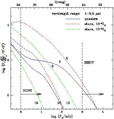
Figure 32. Infrared number counts of quasars (averaged over the wavelength interval of 1-3.5µm) based on the ``simplest quasar model'' of Haiman & Loeb (1999b). The solid curves refer to quasars, while the long/short dashed curves correspond to star clusters with low/high normalization for the star formation efficiency. The curves labeled ``5'' or ``10'' show the cumulative number of objects with redshifts above z = 5 or 10. |
We do, however, expect a substantial intrinsic scatter in the ratio
Mbh / Mgas. Observationally, the
scatter around the
average value of log10(Mbh / L) is 0.3
(Magorrian et al. 1998),
while the standard deviation in
log10(Mbh / Mgas) has
been found to be
~ 0.5. Such an intrinsic
scatter would flatten the predicted quasar luminosity function at the
bright end, where the luminosity function is steeply declining. However,
Haiman & Loeb (1999a)
have shown that the flattening
introduced by the scatter can be compensated for through a modest
reduction in the fitted value for the average ratio between the black
hole mass and halo mass by ~ 50% in the relevant mass range
(108
M
Mbh
1010
M).
In reality, the relation between the black hole and halo masses may be
more complicated than linear. Models with additional free parameters,
such as a non-linear (mass and redshift dependent) relation between
the black hole and halo mass, can also produce acceptable fits to
the observed quasar luminosity function
(Haehnelt et al. 1998).
The nonlinearity in a relation of the type
Mbh  Mhalo
with > 1, may be related to
the physics of the
formation process of low-luminosity quasars
(Haehnelt et al. 1998;
Silk & Rees 1998),
and can be tuned so as to reproduce the black hole
reservoir with its scatter in the local universe
(Cattaneo, Haehnelt,
& Rees 1999).
Recently, a tight correlation between the masses of
black holes and the velocity dispersions of the bulges in which they
reside, , was identified in
nearby galaxies. Ferrarese & Merritt
(2000;
see also
Merritt & Ferrarese
2001)
inferred a correlation of the type
Mbh
4.72±0.36,
based on a selected sample of a dozen galaxies with reliable
Mbh estimates, while
Gebhardt et al. (2000a,
b)
have found a somewhat shallower slope,
Mbh
3.75(±0.3)
based on a
significantly larger sample. A non-linear relation of
Mbh
5
Mhalo5/3 has been predicted by
Silk & Rees (2000)
based on feedback considerations, but the observed
relation also follows naturally in the standard semi-analytic models
of galaxy formation
(Haehnelt &
Kauffmann 2000).
Mhalo
with > 1, may be related to
the physics of the
formation process of low-luminosity quasars
(Haehnelt et al. 1998;
Silk & Rees 1998),
and can be tuned so as to reproduce the black hole
reservoir with its scatter in the local universe
(Cattaneo, Haehnelt,
& Rees 1999).
Recently, a tight correlation between the masses of
black holes and the velocity dispersions of the bulges in which they
reside, , was identified in
nearby galaxies. Ferrarese & Merritt
(2000;
see also
Merritt & Ferrarese
2001)
inferred a correlation of the type
Mbh
4.72±0.36,
based on a selected sample of a dozen galaxies with reliable
Mbh estimates, while
Gebhardt et al. (2000a,
b)
have found a somewhat shallower slope,
Mbh
3.75(±0.3)
based on a
significantly larger sample. A non-linear relation of
Mbh
5
Mhalo5/3 has been predicted by
Silk & Rees (2000)
based on feedback considerations, but the observed
relation also follows naturally in the standard semi-analytic models
of galaxy formation
(Haehnelt &
Kauffmann 2000).
Figure 32 shows the predicted number counts in
the ``simplest model'' described above
(Haiman & Loeb
1999a),
normalized to a
5' × 5' field of view. Figure 32 shows
separately the number per logarithmic flux interval of all objects
with redshifts z > 5 (thin lines), and z > 10 (thick
lines). The
number of detectable sources is high; NGST will be able to probe of
order 100 quasars at z > 10, and ~ 200 quasars at z > 5 per
5' × 5' field of view. The bright-end tail of
the number counts approximately follows a power law, with
dN / dF
F-2.5. The dashed lines show the
corresponding number counts of ``star-clusters'', assuming that each
halo shines due to a starburst that converts a fraction of 2%
(long-dashed) or 20% (short-dashed) of the gas into stars.
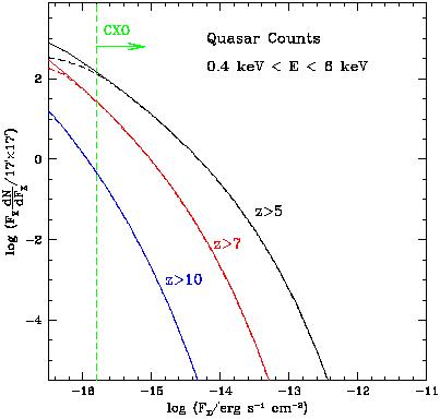
Similar predictions can be made in the X-ray regime. Figure 33 shows the number counts of high-redshift X-ray quasars in the above ``simplest model''. This model fits the X-ray luminosity function of quasars at z ~ 3.5 as observed by ROSAT (Miyaji, Hasinger, & Schmidt 2000), using the same parameters necessary to fit the optical data (Pei 1995). Deep optical or infrared follow-ups on deep images taken with the Chandra X-ray satellite (CXO; see, e.g., Mushotzky et al. 2000; Barger et al. 2000; Giaconni et al. 2000) will be able to test these predictions in the relatively near future.
|
Figure 33.
Total number of quasars with redshift exceeding z = 5, z = 7,
and z = 10 as a function of observed X-ray flux in the CXO
detection band (from
Haiman & Loeb
1999a).
The numbers are normalized per 17' × 17' area of the sky. The
solid curves
correspond to a cutoff in circular velocity for the host halos of
vcirc |
The ``simplest model'' mentioned above predicts that black holes and stars make comparable contributions to the ionizing background prior to reionization. Consequently, the reionization of hydrogen and helium is predicted to occur roughly at the same epoch. A definitive identification of the He2 reionization redshift will provide another powerful test of this model. Further constraints on the lifetime of the active phase of quasars may be provided by future measurements of the clustering properties of quasars (Haehnelt et al. 1998; Martini & Weinberg 2001; Haiman & Hui 2000).
The detection of galaxies and quasars becomes increasingly difficult
at a higher redshift. This results both from the increase in the
luminosity distance and the decrease in the average galaxy mass with
increasing redshift. It therefore becomes advantageous to search for
transient sources, such as supernovae or
 -ray bursts, as
signposts of high-redshift galaxies
(Miralda-Escudé
& Rees 1997).
Prior to or during the epoch of reionization, such sources are
likely to outshine their host galaxies.
-ray bursts, as
signposts of high-redshift galaxies
(Miralda-Escudé
& Rees 1997).
Prior to or during the epoch of reionization, such sources are
likely to outshine their host galaxies.
The metals detected in the IGM (see Section 7.2)
signal the
existence of supernova (SN) explosions at redshifts z
5. Since
each SN produces an average of
~ 1M of
heavy elements
(Woosley & Weaver
1995),
the inferred metallicity of the IGM,
ZIGM, implies that there should be a supernova at
z 5 for each
~ 1.7 × 10⁴
M ×
(ZIGM/10-2.5
Z)-1
of baryons in the universe. We can therefore estimate
the total supernova rate, on the entire sky, necessary to produce
these metals at z ~ 5. Consider all SNe which are observed over a
time interval  t on
the whole sky. Due to the cosmic time
dilation, they correspond to a narrow redshift shell centered at the
observer of proper width
ct /
(1 + z). In a flat
m = 0.3
cosmology, the total mass of baryons in a narrow redshift shell of
width ct /
(1 + z) around z = 5 is
~ [4
t on
the whole sky. Due to the cosmic time
dilation, they correspond to a narrow redshift shell centered at the
observer of proper width
ct /
(1 + z). In a flat
m = 0.3
cosmology, the total mass of baryons in a narrow redshift shell of
width ct /
(1 + z) around z = 5 is
~ [4 (1 + z)-3
(1.8c / H0)2 c
t] ×
[b
(3H02 /
8G)(1 +
z)3] = 4.9 c3
b
t /
G. Hence, for h = 0.7 the
total supernova rate across the entire sky at z
5 is estimated to be
(Miralda-Escudé
& Rees 1997),
(1 + z)-3
(1.8c / H0)2 c
t] ×
[b
(3H02 /
8G)(1 +
z)3] = 4.9 c3
b
t /
G. Hence, for h = 0.7 the
total supernova rate across the entire sky at z
5 is estimated to be
(Miralda-Escudé
& Rees 1997),
| (102) |
or roughly one SN per square arcminute per year.
The actual SN rate at a given observed flux threshold is determined by
the star formation rate per unit comoving volume as a function of
redshift and the initial mass function of stars
(Madau, della Valle,
& Panagia 1998;
Woods & Loeb 1998;
Sullivan et al. 2000).
To derive the relevant expression for flux-limited observations, we
consider a general population of transient sources which are standard
candles in peak flux and are characterized by a comoving rate per unit
volume R(z). The observed number of new events per unit time
brighter than flux
F at observed
wavelength  for such a
population is given by
for such a
population is given by
| (103) |
where
zmax(F, ) is the
maximum redshift at which a source will appear brighter than
F at an observed
wavelength = c /
, and
dVc is the cosmology-dependent comoving
volume element corresponding to a redshift interval dz. The above
integrand includes the (1 + z) reduction in the apparent rate due to
the cosmic time dilation.
Figure 34 shows the predicted SN rate as a function of
limiting flux in various bands
(Woods & Loeb 1998),
based on the
comoving star formation rate as a function of redshift that was
determined empirically by
Madau (1997).
The actual star formation rate
may be somewhat higher due to corrections for dust extinction (for a
recent compilation of current data, see
Blain & Natarajan
2000).
The dashed lines correspond to Type Ia SNe and the dotted lines to Type II
SNe. For comparison, the solid lines indicate two crude estimates for
the rate of
-ray burst
afterglows, which are discussed in detail in the next section.

|
Figure 34.
Predicted cumulative rate
|
Equation (103) is appropriate for a threshold
experiment, one which monitors the sky continuously and triggers when
the detected flux exceeds a certain value, and hence identifies the
most distant sources only when they are near their peak flux. For
search strategies which involve taking a series of ``snapshots'' of a
field and looking for variations in the flux of sources in successive
images, one does not necessarily detect most sources near their peak
flux. In this case, the total number of events (i.e., not
per unit time) brighter than
F at observed
wavelength is given by
| (104) |
where t*(z;
F,
) is the rest-frame duration over
which an event will be brighter than the limiting flux
F at
redshift z. This is a naive estimate of the so-called ``control
time''; in practice, the effective duration over which an event can be
observed is shorter, owing to the image subtraction technique, host
galaxy magnitudes, and a number of other effects which reduce the
detection efficiency
(Pain et al. 1996).
Figure 35 shows the
predicted number counts of SNe as a function of limiting flux for the
parameters used in Figure 34
(Woods & Loeb 1998).

|
Figure 35.
Cumulative number counts N( >
F |
Supernovae also produce dust which could process the emission spectrum
of galaxies. Although produced in galaxies, the dust may be expelled
together with the metals out of galaxies by supernova-driven winds.
Loeb & Haiman (1997)
have shown that if each supernova produces
~ 0.3 M of
Galactic dust, and some of the dust is expelled
together with metals out of the shallow potential wells of the early
dwarf galaxies, then the optical depth for extinction by intergalactic
dust may reach a few tenths at z ~ 10 for observed wavelengths of
~ 0.5-1 µm [see
Todini & Ferrara
(2000)
for a detailed
discussion on the production of dust in primordial Type II SNe]. The
opacity in fact peaks in this wavelength band since at z ~ 10 it
corresponds to rest-frame UV, where normal dust extinction is most
effective. In these estimates, the amplitude of the opacity is
calibrated based on the observed metallicity of the IGM at z
5.
The intergalactic dust absorbs the UV background at the reionization
epoch and re-radiates it at longer wavelengths. The flux and spectrum
of the infrared background which is produced at each redshift depends
sensitively on the distribution of dust around the ionizing sources,
since the deviation of the dust temperature from the microwave
background temperature depends on the local flux of UV radiation that
it is exposed to. For reasonable choices of parameters, dust could
lead to a significant spectral distortion of the microwave background
spectrum that could be measured by a future spectral mission, going
beyond the upper limit derived by the COBE satellite
(Fixsen et al. 1996).
The metals produced by supernovae may also yield strong molecular line
emission.
Silk & Spaans (1997)
pointed out that the rotational line
emission of CO by starburst galaxies is enhanced at high redshift due
to the increasing temperature of the cosmic microwave background,
which affects the thermal balance and the level populations of the
atomic and molecular species. They found that the future Millimeter
Array (MMA) could detect a starburst galaxy with a star formation rate
of ~ 30 M
yr-1 equally well at z = 5 and z = 30
because of the increasing cosmic microwave background temperature with
redshift. Line emission may therefore be a more powerful probe of the
first bright galaxies than continuum emission by dust.
The past decade has seen major observational breakthroughs in the study of Gamma Ray Burst (GRB) sources. The Burst and Transient Source Experiment (BATSE) on board the Compton Gamma Ray Observatory (Meegan et al. 1992) showed that the GRB population is distributed isotropically across the sky, and that there is a deficiency of faint GRBs relative to a Euclidean distribution. These were the first observational clues indicating a cosmological distance scale for GRBs. The localization of GRBs by X-ray observations with the BeppoSAX satellite (Costa et al. 1997) allowed the detection of afterglow emission at optical (e.g., van Paradijs et al. 1997) and radio (e.g., Frail et al. 1997) wavelengths up to more than a year following the events (Fruchter et al. 1999; Frail et al. 2000). The afterglow emission is characterized by a broken power-law spectrum with a peak frequency that declines with time. The radiation is well-fitted by a model consisting of synchrotron emission from a decelerating blast wave (Blandford & McKee 1976), created by the GRB explosion in an ambient medium, with a density comparable to that of the interstellar medium of galaxies (Waxman 1997; Sari, Piran, & Narayan 1998; Wijers & Galama 1999; Mészáros 1999; but see also Chevalier & Li 2000). The detection of spectral features, such as metal absorption lines in some optical afterglows (Metzger et al. 1997) and emission lines from host galaxies (Kulkarni et al. 2000), allowed an unambiguous identification of the cosmological distance-scale to these sources.
The nature of the central engine of GRBs is still unknown. Since the inferred energy release, in cases where it can be securely calibrated (Freedman & Waxman 2001; Frail et al. 2000), is comparable to that in a supernova, ~ 1051 erg, most popular models relate GRBs to stellar remnants such as neutron stars or black holes (Eichler et al. 1989; Narayan, Paczynski, & Piran 1992; Paczynski 1991; Usov 1992; Mochkovitch et al. 1993; Paczynski 1998; MacFadyen & Woosley 1999). Recently it has been claimed that the late evolution of some rapidly declining optical afterglows shows a component which is possibly associated with supernova emission (e.g., Bloom et al. 1999; Reichart 1999). If the supernova association is confirmed by detailed spectra of future afterglows, the GRB phenomenon will be linked to the terminal evolution of massive stars.
Any association of GRBs with the formation of single compact stars implies that the GRB rate should trace the star formation history of the universe (Totani 1997; Sahu et al. 1997; Wijers et al. 1998; but see Krumholz, Thorsett & Harrison 1998). Owing to their high brightness, GRB afterglows could in principle be detected out to exceedingly high redshifts. Just as for quasars, the broad-band emission of GRB afterglows can be used to probe the absorption properties of the IGM out to the reionization epoch at redshift z ~ 10. Lamb & Reichart (2000) extrapolated the observed gamma-ray and afterglow spectra of known GRBs to high redshifts and emphasized the important role that their detection could play in probing the IGM (see also Miralda-Escudé 1998). In particular, the broad-band afterglow emission can be used to probe the ionization and metal-enrichment histories of the intervening intergalactic medium during the epoch of reionization.
Ciardi & Loeb (2000)
showed that unlike other sources (such as
galaxies and quasars), which fade rapidly with increasing redshift,
the observed infrared flux from a GRB afterglow at a fixed observed
age is only a weak function of its redshift
(Figure 36). A
simple scaling of the long-wavelength spectra and the temporal
evolution of afterglows with redshift implies that at a fixed time-lag
after the GRB in the observer's frame, there is only a mild change in
the observed flux at infrared or radio wavelengths with
increasing redshift. This results in part from the fact that
afterglows are brighter at earlier times, and that a given observed
time refers to an earlier intrinsic time in the source frame as the
source redshift increases. The ``apparent brightening'' of GRB
afterglows with redshift could be further enhanced by the expected
increase with redshift of the mean density of the interstellar medium
of galaxies
(Wood & Loeb 2000).
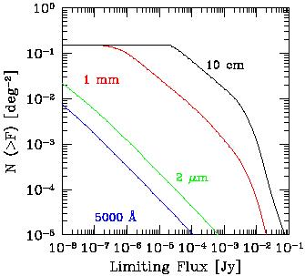
Figure 37 shows the expected
number counts of GRB afterglows, assuming that the GRB rate is
proportional to the star formation rate and that the characteristic
energy output of GRBs is ~ 1052 erg and is
isotropic. The figure implies that at any time there should be of
order ~ 15 GRBs with redshifts z
5 across the sky which are
brighter than ~ 100 nJy at an observed wavelength of ~
2µm. The infrared spectrum of these sources could be
measured with
NGST as a follow-up on their early X-ray localization with
-ray or X-ray
detectors. Prior to reionization, the spectrum
of GRB afterglows could reveal the long sought-after Gunn-Peterson trough
(Gunn & Peterson
1965)
due to absorption by the neutral intergalactic medium.

|
Figure 36.
Observed flux from a
|
The predicted GRB rate and flux are subject to uncertainties regarding
the beaming of the emission. The beaming angle may vary with observed
time due to the decline with time of the Lorentz factor
(t) of
the emitting material. As long as the Lorentz factor is significantly
larger than the inverse of the beaming angle (i.e.,
-1), the
afterglow flux behaves as if it were emitted by a
spherically-symmetric fireball with the same explosion energy per unit
solid angle. However, the lightcurve changes as soon as
declines below
-1, due to the
lateral expansion of the jet
(Rhoads 1997,
1999a,
b;
Panaitescu &
Meszaros 1999).
Finally, the
isotropization of the energy ends when the expansion becomes
sub-relativistic, at which point the remnant recovers the
spherically-symmetric Sedov-Taylor solution
(Sedov 1946,
1959;
Taylor 1950)
with the total remaining energy. When
~ 1, the
emission occurs from a roughly spherical fireball with the effective
explosion energy per solid angle reduced by a factor of
(2
2 /
4) relative to that at early
times, representing the
fraction of sky around the GRB source which is illuminated by the
initial two (opposing) jets of angular radius
(see
Ciardi & Loeb 2000
for the impact of this effect on the number counts). The
calibration of the GRB event rate per comoving volume, based on the
number counts of GRBs
(Wijers et al. 1998),
is inversely proportional to this factor.
|
Figure 37. Predicted number of GRB afterglows per square degree with observed flux greater than F, at several different observed wavelengths (from Ciardi & Loeb 2000). From right to left, the observed wavelength equals 10 cm, 1 mm, 2 µm and 5000 Å. |
The main difficulty in using GRBs as probes of the high-redshift
universe is that they are rare, and hence their detection requires
surveys which cover a wide area of the sky. The simplest strategy for
identifying high-redshift afterglows is through all-sky surveys in the
-ray or X-ray
regimes. In particular, detection of
high-redshift sources will become feasible with the high trigger rate
provided by the forthcoming Swift satellite, to be launched in
2003 (see
http://swift.gsfc.nasa.gov/, for more
details). Swift is expected to localize ~300 GRBs per year, and
to re-point within 20-70 seconds its on-board X-ray and UV-optical
instrumentation for continued afterglow studies. The high-resolution
GRB coordinates obtained by Swift will be transmitted to Earth
within ~ 50 seconds. Deep follow-up observations will then be
feasible from the ground or using the highly-sensitive infrared
instruments on board NGST. Swift will be sufficiently
sensitive to trigger on the
-ray emission
from GRBs at
redshifts z 10
(Lamb & Reichart
2000).
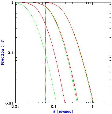
8.3. Distribution of Disk Sizes
Given the distribution of disk sizes at each value of halo mass and
redshift (Section 5.1) and the number counts
of galaxies (Section 8.2.1), we derive the
predicted size distribution of galactic
disks. Note that although frequent mergers at high redshift may
disrupt these disks and alter the morphologies of galaxies, the
characteristic sizes of galaxies will likely not change
dramatically. We show in Figure 38 [an updated
version of Figure 6 of
Barkana & Loeb
(2000a)]
the distribution of galactic disk
sizes at various redshifts, in the
CDM model (with parameters
given at the end of Section 1). Given
in arcseconds, each
curve shows the fraction of the total number counts contributed by
sources larger than . The
diameter is measured out to
one exponential scale length. We show three pairs of curves, at z = 2,
z = 5 and z = 10 (from right to left). Each pair includes the
distribution for all galaxies (dashed line), and for galaxies
detectable by NGST (solid line) with a limiting point source flux
of 0.25 nJy and with an efficiency
= 10% assumed for the
galaxies. The vertical dotted line indicates the expected NGST
resolution of 0".06.
|
Figure 38.
Distribution of galactic disk sizes at various redshifts, in
the |
Among detectable galaxies, the typical diameter decreases from
0".22 at z = 2 to 0".10 at z = 5 and 0".05 at
z = 10. Note that in
CDM (with
m = 0.3) the angular
diameter distance (in units of c / H0) actually
decreases from 0.40
at z = 2 to 0.30 at z = 5 and 0.20 at z =
10. Galaxies are still
typically smaller at the higher redshifts because a halo of a given
mass is denser, and thus smaller, at higher redshift, and furthermore
the typical halo mass is larger at low redshift due to the growth of
cosmic structure with time. At z = 10, the distribution of detectable
galaxies is biased, relative to the distribution of all galaxies,
toward large galaxies, since NGST can only detect the brightest
galaxies. The brightest galaxies tend to lie in the most massive and
therefore largest halos, and this trend dominates over the higher
detection threshold needed for an extended source compared to a point
source (Section 8.1).
Clearly, the angular resolution of NGST will be sufficiently high to resolve most galaxies. For example, NGST should resolve approximately 35% of z = 10 galaxies, 80% of z = 5 galaxies, and all but 1% of z = 2 galaxies. This implies that the shapes of these high-redshift galaxies can be studied with NGST. It also means that the high resolution of NGST is crucial in making the majority of sources on the sky useful for weak lensing studies (although a mosaic of images is required for good statistics; see also the following subsection).
Detailed studies of gravitational lenses have provided a wealth of information on galaxies, both through modeling of individual lens systems (e.g., Schneider, Ehlers, & Falco 1992; Blandford & Narayan 1992) and from the statistical properties of multiply imaged sources (e.g., Turner, Ostriker, & Gott 1984; Maoz & Rix 1993; Kochanek 1996).
The ability to observe large numbers of high-redshift objects promises to greatly extend gravitational lensing studies. Due to the increased path length along the line of sight to the most distant sources, their probability for being lensed is expected to be the highest among all possible sources. Sources at z > 10 will often be lensed by z > 2 galaxies, whose masses can then be determined with lens modeling. Similarly, the shape distortions (or weak lensing) caused by foreground clusters of galaxies will be used to determine the mass distributions of less massive and higher redshift clusters than currently feasible. In addition, it will be fruitful to exploit the magnification of the sources to resolve and study more distant galaxies than otherwise possible.
These applications have been explored by Schneider & Kneib (1998), who investigated weak lensing, and by Barkana & Loeb (2000a), who focused on strong lensing. Schneider & Kneib (1998) noted that the ability of NGST to take deeper exposures than is possible with current instruments will increase the observed density of sources on the sky, particularly of those at high redshifts. The large increase (by ~ 2 orders of magnitude over current surveys) may allow such applications as a detailed weak lensing mapping of substructure in clusters. Obviously, the source galaxies must be well resolved to allow an accurate shape measurement. Barkana & Loeb (2000a) estimated the size distribution of galactic disks (see Section 8.3) and showed that with its expected ~ 0".06 resolution, NGST should resolve most galaxies even at z ~ 10.
The probability for strong gravitational lensing depends on the abundance of lenses, their mass profiles, and the angular diameter distances among the source, the lens and the observer. The statistics of existing lens surveys have been used at low redshifts to constrain the cosmological constant (for the most detailed work see Kochanek 1996, and references therein), although substantial uncertainties remain regarding the luminosity function of early-type galaxies and their dark matter content. Given the early stage of observations of the redshift evolution of galaxies and their dark halos, a theoretical approach based on the Press-Schechter mass function can be used to estimate the lensing rate. This approach has been used in the past for calculating lensing statistics at low redshifts, with an emphasis on lenses with image separations above 5" (Narayan & White 1988; Kochanek 1995; Maoz et al. 1997; Nakamura & Suto 1997; Phillips, Browne, & Wilkinson 2001; Ofek et al. 2000) or on the lensing rates of supernovae (Porciani & Madau 2000; Marri et al. 2000).
The probability for producing multiple images of a source at a redshift zS, due to gravitational lensing by lenses with density distributed as in a singular isothermal sphere, is obtained by integrating over lens redshift zL the differential optical depth (Turner, Ostriker, & Gott 1984; Fukugita et al. 1992)
| (105) |
in terms of the comoving density of lenses n, velocity
dispersion ,
look-back time t, and angular diameter
distances D among the observer, lens and source. More generally we
replace n4 by
| (106) |
where dn/dM is the Press-Schechter halo
mass function. It is assumed that
(M, z) =
Vc(M, z) /
 2
and that the circular velocity Vc(M, z)
corresponding to a halo of a
given mass is given by equation (25).
2
and that the circular velocity Vc(M, z)
corresponding to a halo of a
given mass is given by equation (25).
The CDM model (with
m = 0.3) yields a
lensing optical depth
(Barkana & Loeb 2000a)
of ~ 1% for sources at
zS = 10. The fraction of lensed sources in an actual
survey is enhanced, however, by the so-called magnification bias. At a given
observed flux level, unlensed sources compete with lensed sources that
are intrinsically fainter. Since fainter galaxies are more numerous,
the fraction of lenses in an observed sample is larger than the
optical depth value given above. The expected slope of the luminosity
function of the early sources (Section 8.2) suggests
an additional
magnification bias of order 5, bringing the fraction of lensed sources
at zS = 10 to ~ 5%. The lensed fraction decreases to ~ 3%
at z = 5. With the magnification bias estimated separately for each
source population, the expected number of detected multiply-imaged
sources per field of view of NGST (which we assume to be
4' × 4') is roughly 5 for z > 10 quasars, 10 for z > 5
quasars, 10 for z > 10 galaxies, and 100 for z > 5
galaxies.
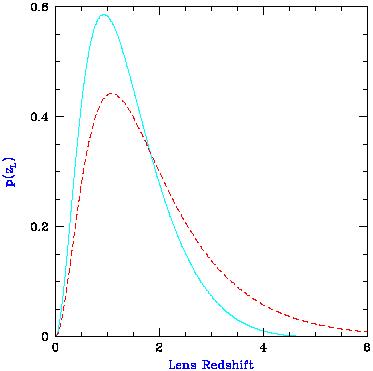
High-redshift sources will tend to be lensed by galaxies at relatively high redshifts. In Figure 39 (adopted from Figure 2 of Barkana & Loeb 2000a) we show the lens redshift probability density p(zL), defined so that the fraction of lenses between zL and zL + dzL is p(zL) dzL. We consider a source at zS = 5 (solid curve) or at zS = 10 (dashed curve). The curves peak around zL = 1, but in each case a significant fraction of the lenses are above redshift 2: 20% for zS = 5 and 36% for zS = 10.
|
Figure 39.
Distribution of lens redshifts for a fixed source redshift,
for Press-Schechter halos in
|
The multiple images of lensed high-redshift sources should be easily resolvable. Indeed, image separations are typically reduced by a factor of only 2-3 between zS = 2 and zS = 10, with the reduction almost entirely due to redshift evolution in the characteristic mass of the lenses. With a typical separation of 0.5-1" for zS = 10, a large majority of lenses should be resolved given the NGST resolution of ~ 0".06.
Lensed sources may be difficult to detect if their images overlap the lensing galaxy, and if the lensing galaxy has a higher surface brightness. Although the surface brightness of a background source will typically be somewhat lower than that of the foreground lens (Barkana & Loeb 2000a), the lensed images should be detectable since (i) the image center will typically be some distance from the lens center, of order half the image separation, and (ii) the younger stellar population and higher redshift of the source will make its colors different from those of the lens galaxy, permitting an easy separation of the two in multi-color observations. These helpful features are evident in the currently known systems which feature galaxy-galaxy strong lensing. These include two four-image `Einstein cross' gravitational lenses and other lens candidates discovered by Ratnatunga et al. (1999) in the Hubble Space Telescope Medium Deep Survey, and a lensed three-image arc detected in the Hubble Deep Field South and studied in detail by Barkana et al. (1999).
6 Model spectra of star-forming galaxies were obtained from http://www.stsci.edu/science/starburst99/. Back.
7 Note that
Fps
is the total spectral flux of the source, not just
the portion contained within the aperture.
Back.
8 We obtained the flux limit using the NGST calculator at http://www.ngst.stsci.edu/nms/main/. Back.
9 Note that the post-reionization threshold was not included in the original discussion of Haiman & Loeb (1998). Back.
 50
km s-1, the dashed curves to a cutoff
of vcirc
50
km s-1, the dashed curves to a cutoff
of vcirc  ( >
F
( >
F