


B.4.3. Constraining the Monopole
The most frustrating aspect of lens modeling is that it is very difficult to
constrain the monopole. If we take a simple lens and fit it with any
of the parametric models from Section B.4.1,
it will be possible to obtain a good fit provided the central surface
density of the model is high enough to avoid the formation of a central
image. As usual, it is simplest to begin understanding the problem with
a circular, two-image lens whose images lie
at radii  A
and B from
the lens center (Fig. B.20).
The lens equation (B.4) constrains the deflections so that
the two images correspond to the same source position,
A
and B from
the lens center (Fig. B.20).
The lens equation (B.4) constrains the deflections so that
the two images correspond to the same source position,
 |
(B.65) |
where the sign changes appear because the images are on opposite
sides of the lens. Recall that for the power-law lens model,
 () = bn-1
2-n
(Eqn. B.9), so we can easily solve
the constraint equation to determine the Einstein radius of the lens,
() = bn-1
2-n
(Eqn. B.9), so we can easily solve
the constraint equation to determine the Einstein radius of the lens,
 |
(B.66) |
in terms of the image positions. In the limit of an SIS (n = 2) the
Einstein radius is the arithmetic mean,
b = (A
+ B) / 2,
and in the limit of a point source (n
 3), it is the
geometric mean,
b = (A
B)1/2, of the image radii.
More generally, for any deflection profile
() = b
f(), the two
images simply determine the mass scale
b = (A
+ B) /
(f(A)
+ f(B)).
3), it is the
geometric mean,
b = (A
B)1/2, of the image radii.
More generally, for any deflection profile
() = b
f(), the two
images simply determine the mass scale
b = (A
+ B) /
(f(A)
+ f(B)).
There are two important lessons here.
First, the location of the tangential critical line is determined
fairly accurately independent of the mass profile. We may only
be able to determine the mass scale, but it is the most accurate
measurement of galaxy masses available to astronomy. The dependence
of the mass inside the Einstein radius on the shape of the
deflection profile is weak, with fractional differences between
profiles being of order ( /
<>)2 /
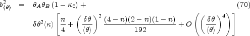
8 where
=
A -
B
and <> =
(A +
B) / 2
(i.e. if the images have similar radii, the difference beween the arthmetic
and geometric mean is small).
Second, it is going to be very difficult to determine radial mass
distributions. In this example there is a perfect degeneracy
between the exact location of the tangential critical line b and
the exponent n. In theory, this is broken by the flux ratio
of the images. However, a simple two-image lens has too few
constraints even with perfectly measured flux ratios because a realistic
lens model must also include some freedom in the angular structure of
the lens. For a simple four-image lens, there begin to be enough
constraints but the images all have similar radii, making the flux
ratios relatively insensitive to changes in the monopole. Combined with
the systematic uncertainties in flux ratios, they are not useful for
this purpose.
/
<>)2 /
8 where
=
A -
B
and <> =
(A +
B) / 2
(i.e. if the images have similar radii, the difference beween the arthmetic
and geometric mean is small).
Second, it is going to be very difficult to determine radial mass
distributions. In this example there is a perfect degeneracy
between the exact location of the tangential critical line b and
the exponent n. In theory, this is broken by the flux ratio
of the images. However, a simple two-image lens has too few
constraints even with perfectly measured flux ratios because a realistic
lens model must also include some freedom in the angular structure of
the lens. For a simple four-image lens, there begin to be enough
constraints but the images all have similar radii, making the flux
ratios relatively insensitive to changes in the monopole. Combined with
the systematic uncertainties in flux ratios, they are not useful for
this purpose.
 |
Figure B.20. A schematic diagram of a
two-image lens. The lens galaxy lies at the origin
with two images A and B at radii
|
This example also leads to the major misapprehension about lens
models and radial mass distributions, in that the constraints
appear to lead to a degeneracy related to the global structure of
the potential (i.e. the exponent n). This is not correct. The
degeneracy is a purely local one that depends only on the structure of the
lens in the annulus defined by the images,
B <
<
A,
as shown in Fig. B.20. To see this we will
rewrite the expression for the bend angle (Eqn. B.3) as
 |
(B.67) |
where bB2 =
2 0B u du
 (u) is the
Einstein radius of the total mass interior to image B, and
(u) is the
Einstein radius of the total mass interior to image B, and
 |
(B.68) |
is the mean surface density in the annulus
B <
u < .
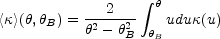
If we now solve the constraint Eqn. B.65 again, we find that
 |
(B.69) |
where
<>AB =
<>
(A,
B) is the
mean density in the annulus
B <
<
A between the
images. Thus, there is a degeneracy between the total mass interior to
image B and the mean surface density (mass) between the two
images. There is no dependence on the distribution of the mass interior
to B, the
distribution of mass between the two images, or on
either the amount or distribution of mass exterior to
A.
This is Gauss' law for gravitational lens models.
If we normalize the mass scale at any point in the interior of the annulus
then the result will appear to depend on the distribution of the mass
simply because the mass must be artificially divided. For example,
suppose we model the surface density locally as a power law
 1-n with a
mean surface density
<> in the annulus
B <
<
A
between the images. The mass inside the mean image radius
<> is
1-n with a
mean surface density
<> in the annulus
B <
<
A
between the images. The mass inside the mean image radius
<> is
 |
(B.70) |
where we have expanded the result in the ratio
/
<> (in fact, the
result as shown is exact for n = 2/3, 1, 2, 4 and 5).
We included in this result an additional, global convergence
0 so that we
can contrast the local degeneracies due to the distribution of matter
between the images with the global degeneracies produced by a infinite
mass sheet. The leading term
A
B is the
Einstein radius
expected for a point mass lens (Eqn. B.65). While the total enclosed
mass (A
B) is fixed,
the mass associated with the lens galaxy
b<>2 must be modified in the presence of a
global convergence by the usual
1 - 0 factor
created by the mass sheet degeneracy (Falco, Gorenstein & Shapiro
[1985]).
The structure of the lens in the annulus leads
to fractional corrections to the mass of order
(
/
<>)2 that
are proportional to
n<> to
lowest order.
Only if you have additional images inside the annulus can you begin
to constrain the structure of the density in the annulus. The constraint
is not, unfortunately, a simple constraint on the density. Suppose
that we see an additional (pair) of images on the Einstein ring at
0, with
B <
0 <
A
This case is simpler than the general case because it divides our
annulus into two sub-annuli (from
B to
0 and from
0 to
A) rather
than three. Since we put the extra
image on the Einstein ring, we know that the mean surface density
interior to 0
is unity (Eqn. B.11). The A and B images then constrain a ratio
 |
(B.71) |
of the average surface densities between the Einstein ring and image B
(<>B0)
and the Einstein ring and image A
(<>A0).
Since a physical distribution must have 0 <
<>A0
< <>B0,
the surface density in the inner sub-annulus must satisfy
 |
(B.72) |
where the lower (upper) bound is found when the density in the outer
sub-annulus is zero (when
<>B0 =
<>A0).
The term
02 -
A
B is the
difference between the measured critical radius
0 and the
critical radius implied by the other two images for a lens with no
density in the annulus (e.g. a point mass),
(A
B)1/2. Suppose we actually
have images formed by an SIS, so
A =
0(1 +
x) and
B =
0(1 -
x) with 0 < x =
 /
0 < 1,
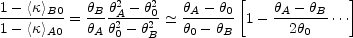
then the lower bound on the density in the inner sub-annulus is
/
0 < 1,
then the lower bound on the density in the inner sub-annulus is
 |
(B.73) |
and the fractional uncertainly in the surface density is unity for
images near the Einstein ring (x
0) and then steadily
diminishes as the A and B images are more asymmetric. If you want
to constrain the monopole, the more asymmetric the configuration the better.
This rule becomes still more important with the introduction of angular
structure.
Fig. B.21 illustrates these issues.
We arbitrarily picked a model consisting of an SIS lens with two sources.
One source is close to the origin and produces images at
A = 1."1
and B =
0."9. The other source is farther from the origin with
images at A =
1."5 and B =
0."5. We then modeled
the lens with either a softened power law (Eqn. B.57) or a
three-dimensional cusp (Eqn. B.58). We did not worry about
the formation of additional images when the core radius becomes too large
or the central cusp is too shallow - this would rule out models with
very large core radii or shallow central cusps. If there were only a
single source, either of these models can fit the data for any values of
the parameters. Once,
however, there are two sources, most of parameter space is ruled out
except for degenerate tracks that look very different for the two mass
models. Along these tracks, the models satisfy the additional constraint
on the surface density given by Eqn. B.71.
The first point to make about Fig. B.21 is the
importance of
carefully defining parameters. The input SIS model has very different
parameters for the two mass models - while the exponent n = 2 is the
same in both cases, the SIS model is the limit
s 0 for
the core radius in the softened power law, but it is the limit
a
 for the break radius in
the cusp model.
Similarly, models with an inner cusp n = 0 will closely resemble
power law models whose exponent n matches the outer exponent m
of the cuspy models. Our frequent failure to explain these similarities
is one reason why lens modeling seems so confusing.
The second point to make about Fig. B.21 is
that the deflection profiles implied by these models are fairly similar
over the annulus bounded by the images. Outside the annulus, particularly
at smaller radii, they start to show very large fractional differences.
Only if we were to add a third set of multiple images or measure a time
delay with a known value of H0 would the
parameter degeneracy begin to be broken.
for the break radius in
the cusp model.
Similarly, models with an inner cusp n = 0 will closely resemble
power law models whose exponent n matches the outer exponent m
of the cuspy models. Our frequent failure to explain these similarities
is one reason why lens modeling seems so confusing.
The second point to make about Fig. B.21 is
that the deflection profiles implied by these models are fairly similar
over the annulus bounded by the images. Outside the annulus, particularly
at smaller radii, they start to show very large fractional differences.
Only if we were to add a third set of multiple images or measure a time
delay with a known value of H0 would the
parameter degeneracy begin to be broken.
 |
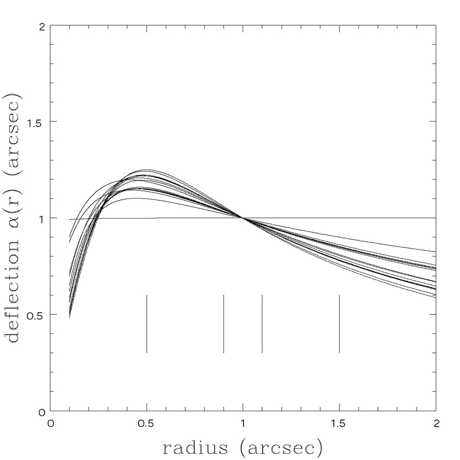 |
Figure 21. Softened power law and cusped model fits to the images produced by an SIS lens with Einstein radius b = 1."0 and two source components located 0."1 and 0."5 from the lens center. In the top panel, the contours show the regions with astrometric fit residuals per image of 0."003 and 0."010. Models with m = 3 cusps so closely overly the m = 4 models that their error contours were not plotted. The bottom panel shows the deflection profiles of the best models at half-integer increments in the exponent n. The SIS model has a constant deflection, and the power-law and cusp models approach it in a sequence of slowly falling deflection profiles. All models agree with the SIS Einstein radius at r = 1."0. The positions of the images are indicated by the vertical bars. |
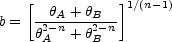
These general results show that studies of how lenses constrain the monopole need the ability to simultaneously vary the mass scale, the surface density of the annulus and possibly the slope of the density profile in the annulus to have the full range of freedom permitted by the data. Most parametric studies constraining the monopole have had two parameters, adjusting the mass scale and a correlated combination of the surface density and slope (e.g. Kochanek [1995a], Impey et al. [1998], Chae, Turnshek & Khersonsky [1998], Barkana et al. [1999], Chae [1999], Cohn et al. [2001], Muñoz et al. [2001], Wucknitz et al. [2004]), although there are exceptions using models with additional degrees of freedom (e.g. Bernstein & Fischer [1999], Keeton et al. [2000], Trott & Webster [2002], Winn, Rusin & Kochanek [2003]). This limitation is probably not a major handicap, because realistic density profiles show a rather limited range of local logarithmic slopes.

 AB
relative to the lens center. For a circular lens
AB
relative to the lens center. For a circular lens