


B.6.2. The Lens Population
The probability that a source has an intervening lens requires a model for the distribution of the lens galaxies. In almost all cases these are based on the luminosity function of local galaxies combined with the assumption that the comoving density of galaxies does not evolve with redshift. Of course luminosity is not mass, so a model for converting the luminosity of a local galaxy into its deflection scale as a lens is a critical part of the process. For our purposes, the distributions of galaxies in luminosity are well-described by a Schechter ([1976]) function,
 |
(B.100) |
The Schechter function has three parameters: a characteristic luminosity
L*
(or absolute magnitude M*), an exponent
 describing the rise at
low luminosity, and a comoving density scale
n*. All these parameters
depend on the type of galaxy being described and the wavelength of the
observations. In general, lens calculations have divided the galaxy
population
into two broad classes: late-type (spiral) galaxies and early-type (E/S0)
galaxies. Over the period lens statistics developed, most luminosity
functions were measured in the blue, where early and late-type galaxies
showed similar characteristic luminosities. The definition of a galaxy type
is a slippery problem - it may be defined by the morphology of the surface
brightness (the traditional method), spectral classifications (the modern
method since it is easy to do in redshift surveys), colors (closely
related to spectra but not identical), and stellar kinematics (ordered
rotational motions versus random motions). Each approach has advantages
and disadvantages,
but it is important to realize that the kinematic definition is the one most
closely related to gravitational lensing and the one never supplied by local
surveys. Fig. B.39 shows an example of a
luminosity function, in this case
K-band infrared luminosity function by Kochanek et al.
([2001],
also Cole et al.
[2001])
where
MK*e = - 23.53 ± 0.06 mag,
n*e = (0.45 ± 0.06) ×
10-2 h3 Mpc-3, and
e = - 0.87
± 0.09 for galaxies which were morphologically early-type galaxies
and MK*l = - 22.98 ± 0.06 mag,
n*l = (1.01 ± 0.13) ×
10-2 h3 Mpc-3, and
l = - 0.92
± 0.10 for galaxies which were morphologically late-type galaxies.
Early-type galaxies are less common but brighter than late-type galaxies
at K-band. It is important to realize that the parameter estimates
of the Schechter function are correlated, as shown in
Fig. B.40, and that it is dangerous to simply
extrapolate them to fainter luminosities than were actually included in
the survey.
describing the rise at
low luminosity, and a comoving density scale
n*. All these parameters
depend on the type of galaxy being described and the wavelength of the
observations. In general, lens calculations have divided the galaxy
population
into two broad classes: late-type (spiral) galaxies and early-type (E/S0)
galaxies. Over the period lens statistics developed, most luminosity
functions were measured in the blue, where early and late-type galaxies
showed similar characteristic luminosities. The definition of a galaxy type
is a slippery problem - it may be defined by the morphology of the surface
brightness (the traditional method), spectral classifications (the modern
method since it is easy to do in redshift surveys), colors (closely
related to spectra but not identical), and stellar kinematics (ordered
rotational motions versus random motions). Each approach has advantages
and disadvantages,
but it is important to realize that the kinematic definition is the one most
closely related to gravitational lensing and the one never supplied by local
surveys. Fig. B.39 shows an example of a
luminosity function, in this case
K-band infrared luminosity function by Kochanek et al.
([2001],
also Cole et al.
[2001])
where
MK*e = - 23.53 ± 0.06 mag,
n*e = (0.45 ± 0.06) ×
10-2 h3 Mpc-3, and
e = - 0.87
± 0.09 for galaxies which were morphologically early-type galaxies
and MK*l = - 22.98 ± 0.06 mag,
n*l = (1.01 ± 0.13) ×
10-2 h3 Mpc-3, and
l = - 0.92
± 0.10 for galaxies which were morphologically late-type galaxies.
Early-type galaxies are less common but brighter than late-type galaxies
at K-band. It is important to realize that the parameter estimates
of the Schechter function are correlated, as shown in
Fig. B.40, and that it is dangerous to simply
extrapolate them to fainter luminosities than were actually included in
the survey.
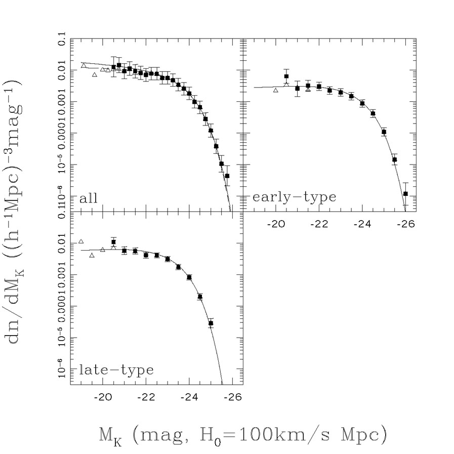 |
Figure B.39. Example of a local galaxy luminosity function. These are the K-band luminosity functions for either all galaxies or by morphological type from Kochanek et al. ([2001]). The curves show the best fit Schechter models for the luminosity functions while the points with error bars show a non-parametric reconstruction. |
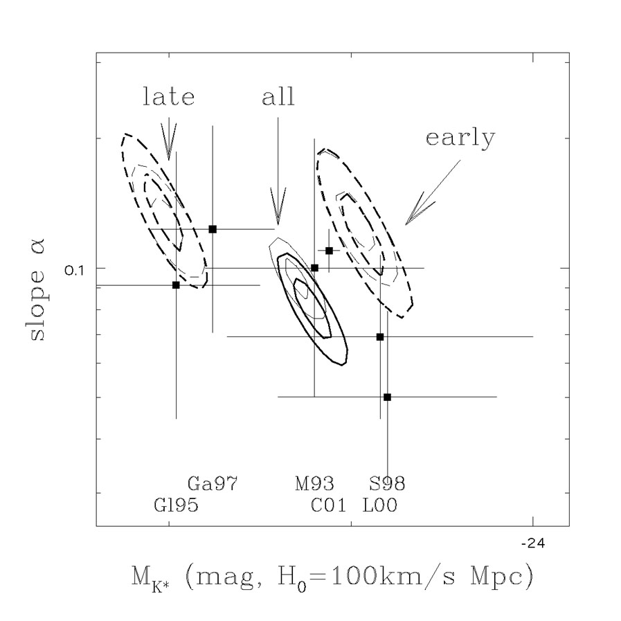 |
Figure B.40. Schechter parameters
|
However, light is not mass, and it is mass which determines lensing
properties.
One approach would simply be to assign a mass-to-light ratio to the galaxies
and to the expected properties of the lenses. This was attempted only
in Maoz & Rix
([1993])
who found that for normal stellar mass
to light ratios it was impossible to reproduce the data (although it is
possible if you adjust the mass-to-light ratio to fit the data, also see
Kochanek
[1996a]).
Instead, most studies convert the
luminosity functions dn / dL into a velocity functions
dn / dv using
the local kinematic properties of galaxies and then relate the stellar
kinematics to the properties of the lens model.
As Fig. B.41
shows (for the same K-band magnitudes of our luminosity function example),
both early-type and late-type galaxies show correlations between luminosity
and velocity. For late-type galaxies there is a tight correlation known
as the Tully-Fisher
([1977])
relation between luminosity L and
circular velocity vc and for early-type galaxies
there is a loose correlation known as the Faber-Jackson
([1976])
relation between luminosity and central velocity dispersion
 v.
Early-type galaxies do show a much tighter correlation known
as the fundamental plane (Dressler et al.
[1987],
Djorgovski & Davis
[1987])
but it is a three-variable correlation
between the velocity dispersion, effective radius and surface brightness
(or luminosity) that we will discuss in
Section B.9. While there is probably some
effect of the FP correlation on lens statistics, it has yet to be
found. For lens calculations, the circular velocity of late-type
galaxies is usually converted into an equivalent
(isotropic) velocity dispersion using
vc = 21/2
v. We can derive
the kinematic relations for the same K-band-selected galaxies used in the
Kochanek et al.
([2001])
luminosity function, finding the Faber-Jackson relation
v.
Early-type galaxies do show a much tighter correlation known
as the fundamental plane (Dressler et al.
[1987],
Djorgovski & Davis
[1987])
but it is a three-variable correlation
between the velocity dispersion, effective radius and surface brightness
(or luminosity) that we will discuss in
Section B.9. While there is probably some
effect of the FP correlation on lens statistics, it has yet to be
found. For lens calculations, the circular velocity of late-type
galaxies is usually converted into an equivalent
(isotropic) velocity dispersion using
vc = 21/2
v. We can derive
the kinematic relations for the same K-band-selected galaxies used in the
Kochanek et al.
([2001])
luminosity function, finding the Faber-Jackson relation
 |
(B.101) |
and the Tully-Fisher relation
 |
(B.102) |
These correlations, when combined with the K-band luminosity function
have the advantage that the magnitude systems for the luminosity
function and the kinematic relations are identical, since magnitude
conversions have caused problems for
a number of lens statistical studies using older photographic luminosity
functions and kinematic relations. For these relations, the characteristic
velocity dispersion of an L* early-type
galaxy is
*e
 209 km/s
while that of an L* late-type galaxy is
*l
143 km/s. These
are fairly typical values even if derived from a completely independent set
of photometric data.
209 km/s
while that of an L* late-type galaxy is
*l
143 km/s. These
are fairly typical values even if derived from a completely independent set
of photometric data.
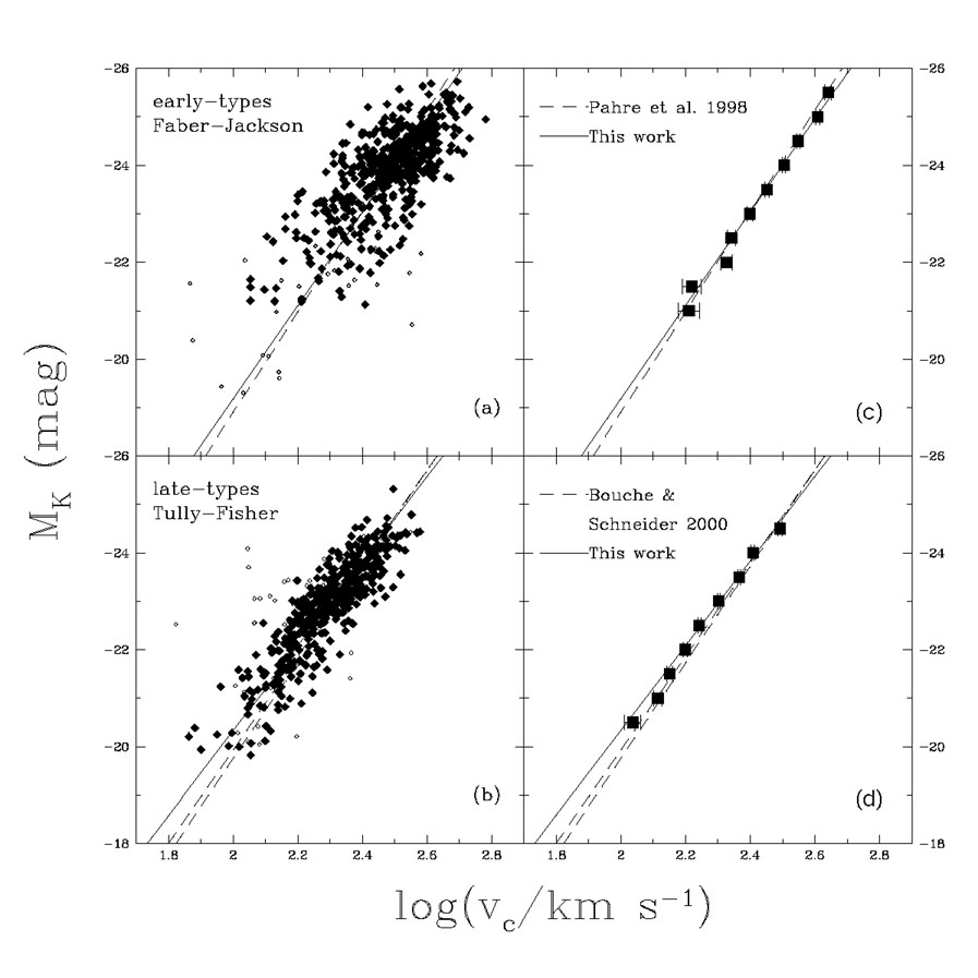 |
Figure B.41. K-band kinematic relations for 2MASS galaxies. The top panels show the Faber-Jackson relation and the bottom panels show the Tully-Fisher relations for 2MASS galaxies with velocity dispersions and circular velocities drawn from the literature. The left hand panels show the individual galaxies, while the right hand galaxies show the mean relations. Note the far larger scatter of the Faber-Jackson relation compared to the Tully-Fisher relation. |
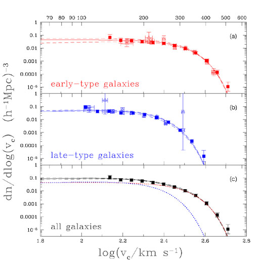 |
Figure B.42. The resulting velocity functions from combining the K-band luminosity functions (Fig. B.39) and kinematic relations (Fig. B.41) for early-type (top), late-type (middle) and all (bottom) galaxies. The points show partially non-parametric estimates of the velocity function based on the binned estimates in the right hand panels of Fig. B.41 rather than power-law fits. Note that early-type galaxies dominate for high circular velocity. |
Both the Faber-Jackson and Tully-Fisher relations are power-law
relations between luminosity and velocity, L /
L*
 (v /
*)
(v /
*) FJ. This allows
a simple variable transformation to convert the luminosity function into a
velocity function,
FJ. This allows
a simple variable transformation to convert the luminosity function into a
velocity function,
 |
(B.103) |
There are three caveats to keep in mind about this variable
change. First, we have converted to the distribution in stellar
velocities, not some underlying velocity
characterizing the dark matter distribution.
Many early studies assumed a fixed transformation
between the characteristic velocity of the stars and the lens model. In
particular, Turner, Ostriker & Gott
([1984])
introduced the assumption
dark =
(3/2)1/2
stars for
an isothermal mass model based on the stellar dynamics
(Jeans equation, Eqn. B.90 and
Section B.4.9)
of a r-3 stellar density distribution in a
r-2 isothermal mass distribution. Kochanek
([1993b],
[1994])
showed that this
oversimplified the dynamics and that if you embed a real stellar luminosity
distribution in an isothermal mass distribution you actually find that
the central stellar velocity dispersion is close to the velocity
dispersion characterizing
the dark matter halo. Fig. B.43 compares the
stellar velocity
dispersion to the dark matter halo dispersion for a Hernquist
distribution of stars in an isothermal mass distribution. Such a
normalization calculation is required for any attempt to match the
observed velocity functions with a particular mass model for the lenses.
Second, in an ideal world, the luminosity function and the kinematic
relations should
be derived from a consistent set of photometric data, while in practice they
rarely are. As we will see shortly, the cross
section for lensing scales roughly as *4, so small errors in
estimates of the characteristic velocity have enormous impacts on the
resulting cosmological results - a 5% velocity calibration error leads
to a 20% error in the lens cross section. Since luminosity functions and
kinematic relations are rarely derived consistently (the exception is
Sheth et al.
[2003]),
the resulting systematic errors creep
into cosmological estimates. Finally, for the early-type galaxies
where the Faber-Jackson kinematic relation has significant scatter,
transforming the luminosity function using the mean relation as we
did in Eqn. B.103 while ignoring the scatter underestimates the number
of high velocity dispersion galaxies (Kochanek
[1994],
Sheth et al.
[2003]).
This leads to underestimates of both
the image separations and the cross sections. The fundamental lesson of
all these issues is that the mass scale of the
lenses should be "self-calibrated" from the observed separation distribution
of the lenses rather than imposed using local observations
(as we discuss below in Section B.6.7).
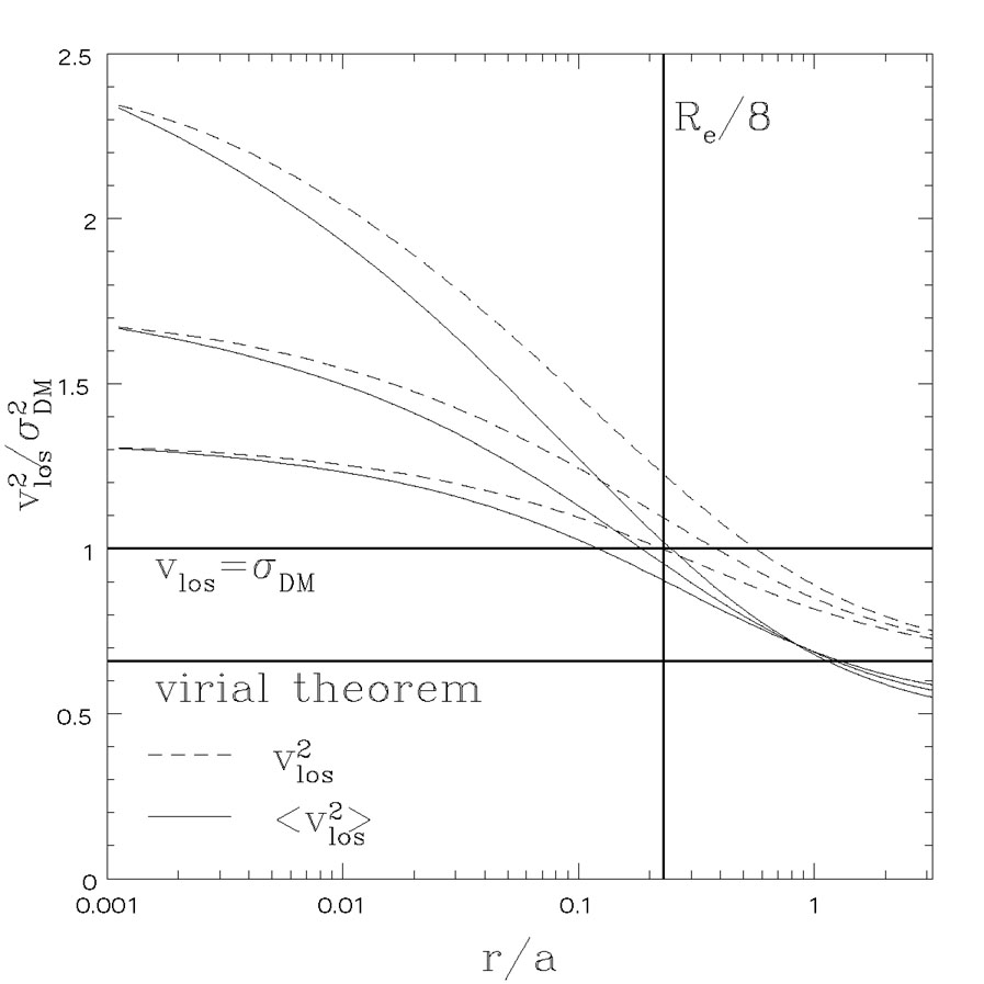 |
Figure B.43. Stellar velocity dispersions
vlos for a Hernquist
distribution of stars in an isothermal halo of dispersion
|
Most lens calculations have assumed that the comoving density of the lenses
does not evolve with redshift. For moderate redshift sources this only
requires little evolution for zl < 1 (mostly
zl < 0.5), but for higher redshift
sources it is important to think about evolution as well.
The exact degree of evolution is the subject of some debate, but a standard
theoretical prediction for the change between now and redshift unity is
shown in Fig. B.44 (see Mitchell et al.
[2004]
and references therein). Because lower mass systems merge to
form higher mass systems as the universe evolves, low mass systems are
expected to be more abundant at higher redshifts while higher mass systems
become less abundant. For the
v ~
* ~
200 km/s galaxies
which dominate lens statistics, the evolution in the number of galaxies is
actually quite modest out to redshift unity, so we would expect galaxy
evolution to have little effect on lens statistics. Higher mass systems
evolve rapidly
and are far less abundant at redshift unity, but these systems will tend to
be group and cluster halos rather than galaxies and the failure of the
baryons to cool in these systems is of greater importance to their
lensing effects than their number evolution (see
Section B.7). There have been
a number of studies examining lens statistics with number evolution
(e.g. Mao
[1991],
Mao & Kochanek
[1994],
Rix et al.
[1994])
and several attempts to use the lens data to constrain the evolution
(Ofek, Rix & Maoz
[2003],
Chae & Mao
[2003],
Davis, Huterer & Krauss
[2003]).
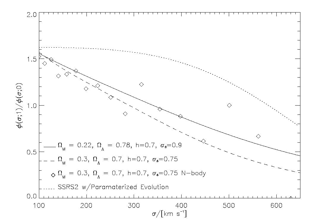 |
Figure B.44. The ratio of the velocity
function of halos at z = 1 to that at z = 0 from Mitchell
et al.
([2004]).
The solid curve shows the expectation for an
|
 = 0.2 (somewhat
radial),
= 0.2 (somewhat
radial), 
