B.9. THE OPTICAL PROPERTIES OF LENS GALAXIES

The optical properties of lens galaxies and the properties of their interstellar medium (ISM) are important for two reasons. First, statistical calculations such as those in Section B.6 rely on lens galaxies obeying the same scaling relations as nearby galaxies and the selection effects depend on the properties of the ISM. Thus, measuring the scaling relations of the observed lenses and the properties of their ISM are an important part of validating these calculations. Second, lenses have a unique advantage for studying the evolution of galaxies because they are the only sample of galaxies selected based on mass rather than luminosity, surface brightness or color. Evolution studies using optically-selected samples will always be subject to strong biases arising from the difficulty of matching nearby galaxies to distant galaxies. Selection by mass rather than light makes the lens samples almost immune to these biases.

Most lens galaxies are early-type galaxies with relatively red colors and few signs of significant on-going star formation (like the 3727Å or 5007Å Oxygen lines). The resulting need to measure absorption line redshifts is one of the reasons that the completeness of the lens redshift measurements is so poor. Locally, early-type galaxies follow a series of correlations which also exist for the lens galaxies and have been explored by Im, Griffiths & Ratnatunga ([1997]), Keeton, Kochanek & Falco ([1998]), Kochanek et al. ([2000]), Rusin et al. ([2003]), Rusin, Kochanek & Keeton ([2003]), van de Ven, van Dokkum & Franx ([2003]), Rusin & Kochanek ([2004]).

The first, crude correlation is the Faber-Jackson relation between velocity dispersion and luminosity used in most lens statistical calculations. A typical local relation is that from Section B.6.2 and shown in Fig.B.41. Most lenses lack directly measured velocity dispersions, but all lenses have a well-determined image separation . For specific mass models the image separation can be converted into an estimate of a velocity dispersion, such as the = 8(_v / c)² D_ds / D_s relation of the SIS, but the precise relationship depends on the mass distribution, the orbital isotropy, the ellipticity and so forth (see Section B.4.9). For the lenses, there is a close relationship between the Faber-Jackson relation and aperture mass-to-light ratios. The image separation, , defines the aperture mass interior to the Einstein ring,

(B.127)

where _c = c² D_s / 4 G D_ds D_d is the critical surface density. By image separation we usually mean either twice the mean distance of the images from the lens galaxy or twice the critical radius of a simple lens model rather than a directly measured image separation because these quantities will be less sensitive to the effects of shear and ellipticity. If we measure the luminosity in the aperture L_ap using (usually) HST, then we know the aperture mass-to-light (M / L) ratio _ap = M_ap / L_ap.

If the mass-to-light ratio varies with radius or with mass, then to compare values of _ap from different lenses we must correct them to a common radius and common mass. If these scalings can be treated as power laws, then we can define a corrected aperture mass to light ratio _* = _ap(D_d^ang / 2R₀)^x where R₀ is a fiducial radius and x is an unknown exponent, and we would expect to find a correlation of the form

(B.128)

where M_abs is the absolute magnitude of the lens (in some band) and a value a 0 indicates that the mass-to-light ratio varies either with mass or with radius. We can then rewrite this in a more familiar form as

(B.129)

where ₀ sets an arbitrary separation scale, _EV (or a more complicated function) determines the evolution of the luminosity with redshift, and _FJ = 4(1 + a) sets the scaling of luminosity with normalized separation defined so that for an SIS lens (where _v²) the exponent _FJ will match the index of the Faber-Jackson relation (Eqn. B.102). Fig. B.64 shows the resulting relation converted to the rest frame B band at redshift zero. The relation is slightly tighter than local estimates of the Faber-Jackson relation, but the scatter is still twice that expected from the measurement errors. The best fit exponent _FJ = 3.29 ± 0.58 (Fig. B.65) is consistent with local estimates and implies a scaling exponent a = - 0.18 ± 0.14 that is marginally non-zero. If the mass-to-light ratio of early-type galaxies increases with mass as M^x, then x = - a = 0.18 ± 0.14 is consistent with estimates from the fundamental plane that more massive early-type galaxies have higher mass-to-light ratios. The solutions also require evolution with _EV = - 0.41 ± 0.21, so that early-type galaxies were brighter in the past. These scalings can also be done in terms of observed magnitudes rather than rest frame magnitudes to provide simple estimation formulas for the apparent magnitudes of lens galaxies in various bands as a function of redshift and separation to an rms accuracy of approximately 0.5 mag (see Rusin et al. [2003]).

Figure B.64. (Top) The "Faber-Jackson" relation for gravitational lenses. The figure compares the observed absolute B magnitude corrected for evolution to that predicted from the equivalent of the Faber-Jackson relation for gravitational lenses (Eqn. B.129). The different point styles indicate whether the lens and source redshifts were directly measured or estimated. From Rusin et al. ([2003]). Figure B.65. (Bottom) The redshift zero absolute B-band magnitude and effective exponent of the "Faber-Jackson" relation L FJ/2 for gravitational lenses.

The significant scatter of the Faber-Jackson relation makes it a crude tool. Early-type galaxies also follow a far tighter correlation known as the fundamental plane (FP, Dressler et al. [1987], Djorgovski & Davis [1987]) between the central, stellar velocity dispersion _c, the effective radius R_e and the mean surface brightness inside the effective radius <SB_e> of the form

(B.130)

where the slope and the zero-point depend on wavelength but the slope 0.32 does not (e.g. Scodeggio et al. [1998], Pahre, de Carvalho & Djorgovski [1998]). Local estimates for the rest frame B-band give = 1.25 and ₀ = - 8.895 - log(h/0.5) (e.g. Bender et al. [1998]). In principle both the zero points and the slopes may evolve with redshift, but all existing studies have assumed fixed slopes and studied only the evolution of the zero point with redshift. For galaxies with velocity dispersion measurements, the basis of the method is that measurement of R_e and _v provides an estimate of the surface brightness the galaxy will have at redshift zero. The difference between the measured surface brightness at the observed redshift and the surface brightness predicted for z = 0 measures the evolution of the stellar populations between the two epochs as a shift in the zero-point . The change in the zero-point is related to the change in the luminosity by L = - 0.4 SB_e = / (2.5). While these estimates are always referred to as a change in the mass-to-light ratio, no real mass measurement enters operationally. If, however, we assume a non-evolving virial mass estimate M = c_{M v}² R_e / G for some constant c_M, then the FP can be rewritten in terms of a mass-to-light ratio,

(B.131)

so that if both and do not evolve, the evolution of the mass-to-light ratio is d log / dz = - (d / dz) / (2.5). Either way of thinking about the FP, either as an empirical estimator of the redshift zero surface brightness or an implicit estimate of the virial mass, leads to the same evolution estimates but alternate ways of thinking about potential systematic errors.

Confusion about applications of lenses to the FP and galaxy evolution usually arise because most gravitational lenses lack direct measurements of the central velocity dispersion. Before addressing this problem, it is worth considering what is done for distant galaxies with direct measurements. The central dispersion appearing in the FP has a specific definition - usually either the velocity dispersion inside the equivalent of a 3."0 aperture in the Coma cluster or the dispersion inside R_e / 8. Measurements for particular galaxies almost never exactly match these definitions, so empirical corrections are applied to adjust the velocity measurements in the observed aperture to the standard aperture. As we explore more distant galaxies, resolution problems mean that the measurement apertures become steadily larger than the standard apertures. The corrections are made with a single, average local relation for all galaxies - implicit in this assumption is that the dynamical structure of the galaxies is homogeneous and non-evolving. This seems reasonable since the minimal scatter around the FP seems to require homogeneity, but says nothing about evolution. These are also the same assumptions used in the lensing analyses.

If early-type galaxies are homogeneous and have mass distributions that are homologous with the luminosity distributions, then there is no difference between the lens FP and the normal kinematic FP, independent of the actual mass distribution of the galaxies (Rusin & Kochanek [2004]). If the mass distributions are homologous, then the mass and velocity dispersion are related by M = c_{M c}² R_e/G where c_M is a constant, _c is the central velocity dispersion (measured in a self-similar aperture like the R_e / 8 aperture used in many local FP studies), and R_e is the effective radius. If we allow the mass-to-light ratio to scale with luminosity as L^x, then the normal FP can be written as

(B.132)

which looks like the local FP (Eqn. B.130) if = 2 / (2x + 1) and = 0.4(x + 1) / (2x + 1) (see Faber et al. [1987]). Thus, the lens galaxy FP will be indistinguishable from the FP provided early-type galaxies are homologous and the slopes can be reproduced by a scaling of the mass-to-light ratio (as they can for x 0.3 given 1.2 and 0.3, e.g., Jorgensen, Franx & Kjaergaard [1996] or Bender et al. [1998]). All the details about the mass distribution, orbital isotropies and the radius interior to which the velocity dispersion is measured enter only through the constant c_M or equivalently from differences between the FP zero point measured locally and with gravitational lenses. In practice, Rusin & Kochanek ([2004]) show that the zero point must be measured to an accuracy significantly better than = 0.1 before there is any sensitivity to the actual mass distribution of the lenses from the FP. Thus, there is no difference between the aperture mass estimates for the FP and its evolution and the normal stellar dynamical approach unless the major assumption underlying both approaches is violated. It also means, perhaps surprisingly, that measuring central velocity dispersions adds almost no new information once these conditions are satisfied.

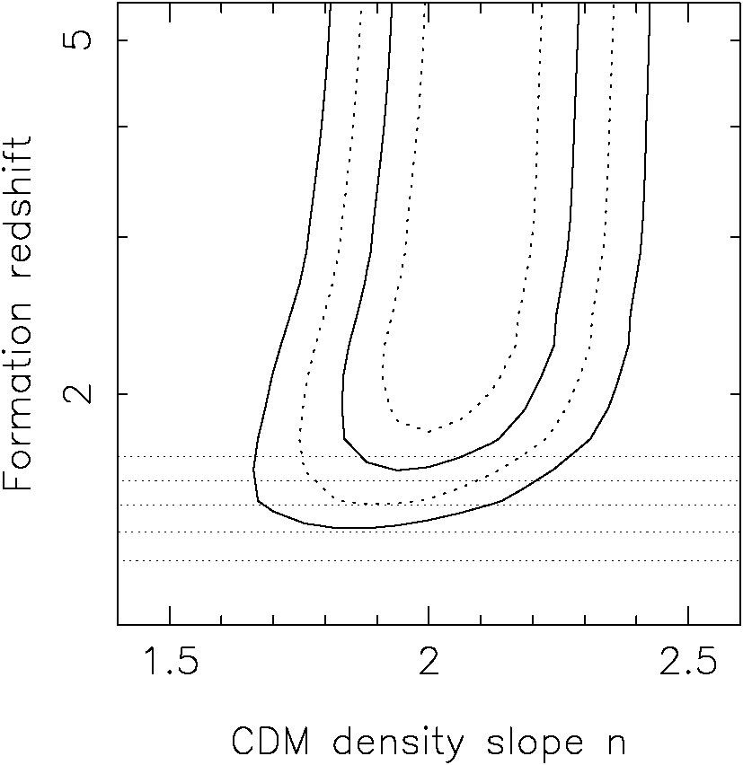
Rusin & Kochanek ([2004]) used the self-similar models we described in Section B.4.8 to estimate the evolution rate and the star formation epoch of the lens galaxies while simultaneously estimating the mass distribution. Thus, the models for the mass include the uncertainties in the evolution and the reverse. Fig. B.66 shows the estimated evolution rate, and Fig. B.67 shows how this is related to a limit on the average star formation epoch <z_f> based on Bruzual & Charlot ([1993], BC96 version) population synthesis models. This estimate is consistent with the earlier estimates by Kochanek et al. ([2000]) and Rusin et al. ([2003]) which used only isothermal lens models, as we would expect. Van de Ven, van Dokkum & Franx ([2003]) found a somewhat lower star formation epoch (<z_f> = 1.8_-0.5^1.4) when analyzing the same data, which can be traced to differences in the analysis. First, by weighting the galaxies by their measurement errors when the scatter is dominated by systematics and by dropping two higher redshift lens galaxies with unknown source redshifts, van de Ven et al. ([2003]) analysis reduces the weight of the higher redshift lens galaxies, which softens the limits on low <z_f>. Second, they used a power law approximation to the stellar evolution tracks which underestimates the evolution rate as you approach the star formation epoch, thereby allowing lower star formation epochs. These two effects leverage a small difference in the evolution rate ¹⁰ into a much more dramatic difference in the estimated star formation epoch. These evolution rates are consistent with estimates for cluster or field ellipticals by (e.g. van Dokkum et al. [1996], [2001], van Dokkum & Franx [2001], van Dokkum & Ellis [2003], Kelson et al. [1997], [2000]), and inconsistent with the much faster evolution rates found by Treu et al. ([2001], [2002]) or Gebhardt et al. ([2003]).

Figure B.66. (Top) Constraints on the B-band luminosity evolution rate d log(M / L)B/dz as a function of the logarithmic density slope n ( r-n) of the galaxy mass distribution. Solid (dashed) contours are the 68% and 95% confidence limits on two parameter (one parameter). These use the self-similar mass models of Eqn. B.89 and are closely related to the fundamental plane. From Rusin & Kochanek ([2004]). Figure B.67. (Bottom) Constraints on the mean star formation epoch <zf> as a function of the logarithmic density slope n ( r-n) of the galaxy mass distribution. Solid (dashed) contours are the 68% and 95% confidence limits on two parameter (one parameter). The horizontal dotted lines mark <zf> = 1.3, 1.4, 1.5, 1.6 and 1.7. The lens sample favors older stellar populations with <zf> > 1.5 at 95% confidence. These use the self-similar mass models of Eqn. B.89 and are closely related to the fundamental plane. From Rusin & Kochanek ([2004]).

¹⁰ Rusin & Kochanek ([2004]) obtained d log(M / L)_B / dz = - 0.50 ± 0.19 including the uncertainties in the mass distribution, Rusin et al. ([2003]) obtained -0.54 ± 0.09 for a fixed SIS model, and van de Ven et al. ([2003]) obtained -0.62 ± 0.13 for a fixed SIS model. Back.