B.4.8. Statistical Constraints on Mass Distributions

Where individual lenses may fail to constrain the mass distribution, ensembles of lenses may succeed. There are two basic ideas behind statistical constraints on mass distributions. The first idea is that models of individual lenses should be weighted by the likelihood of the observed configuration given the model parameters. The second idea is that the statistical properties of lens samples should be homogeneous.

An example of weighting models by the likelihood is the limit on the slopes of central density cusps from the observed absence of central images. Rusin & Ma ([2001]) considered 6 CLASS (see Section B.6) survey radio doubles and computed the probability p_i(n) that lens i would have a detectable third image in the core of the lens assuming power law mass densities R^1-n and including a model for the observational sensitivities and the magnification bias (see Section B.6.6) of the survey. They were only interested in the range n < 2, because as discussed in Section B.3, density cusps with n 2 never have central images. For most of the lenses they considered, it was possible to find models of the 6 lenses that lacked detectable central images over a broad range of density exponents. However, the shallower the cusp, the smaller the probability p_i(n) of producing a lens without a visible central image. For any single lens, p_i(n) varies too little to set a useful bound on the exponent, but the joint probability of the entire sample having no central images, P = _i(1 - p_i(n)), leads to a strong (one-sided) limit that n > 1.78 at 95% confidence (see Fig. B.28). In practice, Keeton ([2003a]) demonstrated that the central stellar densities are sufficiently high to avoid the formation of visible central images in almost all lenses given the dynamic ranges of existing radio observations (i.e. stellar density distributions are sufficiently cuspy), and central black holes can also assist in suppressing the central image (Mao, Witt & Koopmans [2001]). However, the basic idea behind the Rusin & Ma ([2001]) analysis is important and underutilized.

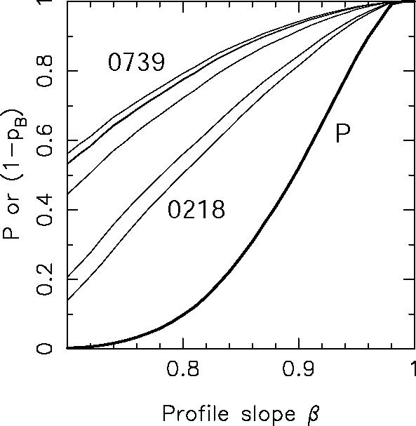Figure B.28. Limits on the central density exponent for power-law density profiles r-n = r-1- from the absence of detectable central images in a sample of 6 CLASS survey radio doubles (Rusin & Ma [2001]). The lighter curves show the limits for the individual lenses with the weakest constraint from B0739+366 and the strongest from B0218+357, and the heavy solid curve shows the joint probability P.

An example of requiring the lenses to be homogeneous is the estimate of the misalignment between the major axis of the luminous lens galaxy and the overall mass distribution by Kochanek ([2002b]). Fig. B.29 shows the misalignment angle _LM = |_L - _M| between the major axis _L of the lens galaxy and the major axis _M of an ellipsoidal mass model for the lens. The particular mass model is unimportant because any single component model of a four-image lens will give a nearly identical value for _M (e.g. Kochanek [1991a], Wambsganss & Paczynski [1994]). The distribution of the misalignment angle _LM is not consistent with the mass and the light being either perfectly correlated or uncorrelated. This is not surprising, because a simple ellipsoidal model determines the position angle of the mean quadrupole moment near the Einstein ring, which is a combination of the quadrupole moment of the lens galaxy, the halo of the lens galaxy, and the local tidal shear (see Section B.4.4). Even if the lens galaxy and the halo were perfectly aligned, we would still find that the orientation of the mean quadrupole would differ from that of the light because of the effects of the tidal shears. 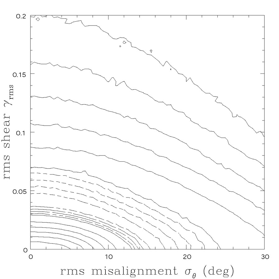We can model this by estimating the probability of reproducing the observed misalignment distribution in terms of the strength of the local tidal shear _rms and the dispersion in in the angle between the major axis of the mass distribution and the light, as shown in Fig. B.30. The observed mismatch can either be produced by having a typical tidal shear of _rms 0.05 or by having a typical misalignment between mass and light of 20°. We know, however, that the typical tidal shear cannot be zero because it can be estimated from the statistics of galaxies (e.g. Keeton, Kochanek & Seljak [1997], Holder & Schechter [2003]). Keeton et al. ([1997]) obtained _rms 0.05, in which case mass must align with light and we obtain an upper limit of 10°. Holder & Schechter ([2003]) argue for a much higher rms shear of _rms = 0.15 based on N-body simulations, which is too high to be consistent with the observed alignment of mass models and the luminous galaxy. One possible explanation (based on the results of White, Hernquist & Springel [2001]) is that Holder & Schechter ([2003]) included parts of the lens galaxy's own halo in their estimate of the external shear. Alternatively, if lens galaxies are more compact than the SIE model used by Kochanek ([2002b]), then the lower surface density <> raises the required shear (since (1 - <>), Eqn. B.78). However, mass distributions similar to constant mass-to-light ratio models of the lenses would be required, which would be inconsistent with shear estimates from simulations in which galaxy masses are dominated by extended dark matter halos.

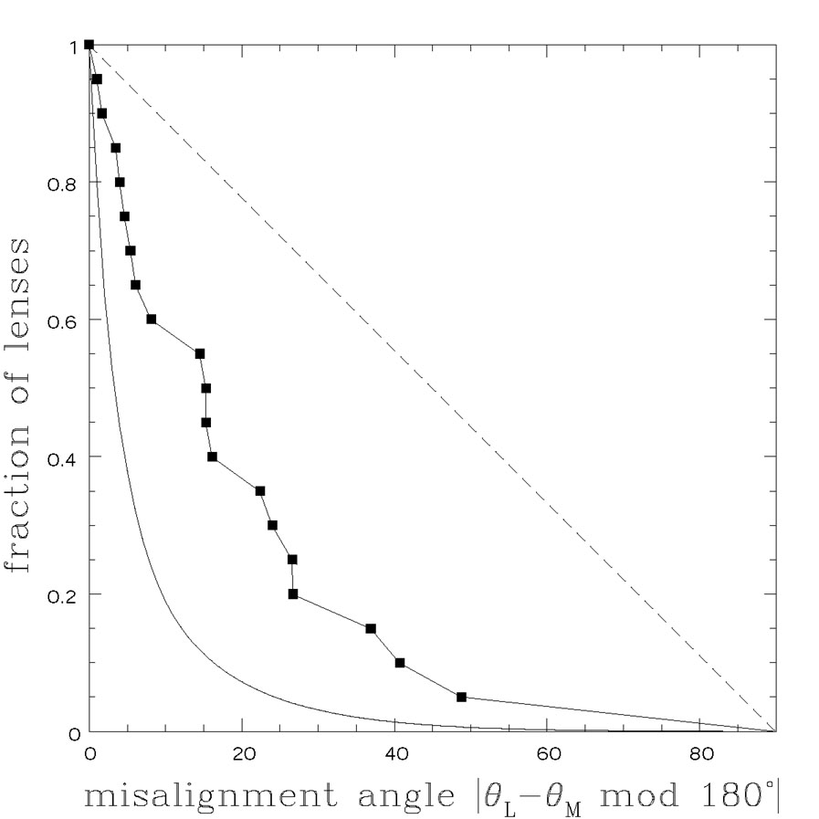Figure B.29. (Top) The integral distribution of misalignment angles LM between the major axes of the lens galaxy and an ellipsoidal lens model (solid curve with points for each lens). If the two angles were completely uncorrelated, the distribution would follow the dashed line. If the two angles were perfectly correlated they would follow the solid curve because of the measurement uncertainties in the two angles. Figure B.30. (Bottom) Logarithmic contours of the probability for matching the distribution of misalignment angles as a function of the rms misalignment between the mass and the light and the typical tidal shear rms. Theoretically we expect tidal shears rms 0.06. The solid contours are spaced by 0.5 dex and the dashed contours are spaced by 0.1 dex relative to the maximum likelihood contour. The differences between dashed contours are not statistically significant, while those between solid contours are statistically significant.

The trade-off between central concentration and shear leads to the the interesting question of where the quadrupole structure of lenses originates. As we discussed in Section B.4.4, we can break up the quadrupole of the mass distribution into the internal quadrupole due to the matter interior to the Einstein ring (Eqn. B.52) and the exterior quadrupole due to the matter outside the Einstein ring (Eqn. B.51). While the internal quadrupole is due only to the lens galaxy, the external quadrupole is a mixture of the quadrupole from the parts of the galaxy outside the Einstein ring (i.e. the dark matter halo) and the tidal shear from the environment. An important fact to remember is that for an isothermal ellipsoid, only f_int = 25% of the quadrupole is due to mass inside the Einstein ring (see Fig. B.22, Section B.4.4)! Turner, Keeton & Kochanek ([2004]) explored this by fitting all the available four-image lenses with an SIS monopole combined with an internal and an external quadrupole. They then computed the fraction of the quadrupole f_int associated with the mass interior to the Einstein ring to find the distribution shown in Fig. B.31. Most four-image lenses seem to be dominated by the external quadrupole, with internal quadrupole fractions below the f_int = 0.25 fraction expected for an isothermal ellipsoid. Lenses clearly in environments with very large tidal shears (e.g. RXJ0911+0551 which is near massive cluster, Bade et al. [1997], Kneib et al. [2000], Morgan et al. [2001] or HE0435-1223 which is near a large galaxy, Wisotzki et al. [2002], see Fig. B.4) show much smaller internal shear fractions. B1608+656 (Myers et al. [1995], Fassnacht et al. [1999]), which has two lens galaxies inside the Einstein ring, shows a significantly higher internal quadrupole fraction. Combined with the close correlation of mass model alignments with the luminous galaxies, this seems to argue for significant dark matter halos aligned with the luminous galaxy, but the final step of quantitatively assembling all the pieces has yet to be done.

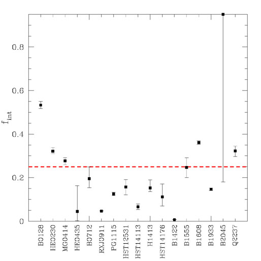Figure B.31. The internal shear fraction fint for the four-image lenses. Each system was fitted by an SIS combined with an internal shear and an external shear and fint = || / (|| + ||) is the fraction of the quadrupole amplitude due to the internal shear. An SIE has fint = 1/4 (see Fig B.22). Most of the quads have fint 1/4 as expected for an SIE in an additional external (tidal) shear field. Objects with very low fint (e.g. HE0435-1223, RXJ0911+0551, B1422+231) have nearby galaxies or clusters generating anomalously large external shears, while objects with anomalously high fint (B1608+656, HE0230-2130, MG0414+0534) tend to have additional lens components like the second lens galaxy of B1608+656. For some systems either the imaging data (e.g. B0128+437) or the models (e.g. B2045+265) do not allow a clear qualitative explanation.

Statistical analyses can also be used to estimate the radial density distribution from samples of lenses which individually cannot. The existence of the fundamental plane (see Section B.9) strongly suggests that the structure of early-type galaxies is fairly homogeneous - in particular it is consistent with galaxies having self-similar mass distributions in the sense that the halo structure can be scaled from the structure of the visible galaxy. As a particular example based on our theoretical expectations, Rusin, Kochanek & Keeton ([2003]) and Rusin & Kochanek ([2004]) modeled the visible galaxy with a Hernquist (Eqn. B.56) model scaled to match the observed effective radius of the lens galaxy, R_e, and then added a cuspy dark matter halo (Eqn. B.59 with a variable inner cusp , = 2 and m = 3) where the inner density cusp ( r^-), the halo break radius r_b and the dark matter fraction f_CDM inside 2R_e were kept as variables. The assumption of self-similarity enters by keeping the ratio r_b / R_e constant, the dark matter fraction f_CDM constant, and then scaling the mass-to-light ratio of the stars L^x with the luminosity. ⁴ We recover the fundamental plane in this model when x 0.25. Putting all the pieces together, the projected mass inside radius R is

(B.89)

where _* is the mass-to-light ratio of the stars in an L_* galaxy, log L(0) = log L(z) - e(z) is the luminosity of the lens galaxy evolved to redshift zero (where we discuss estimates of the evolution rate e(z) in Section B.9), g(x) is the fraction of the light inside dimensionless radius x = R / R_e (g(1) = 1/2) and m_CDM(x) is the dimensionless dark matter mass inside radius x with m_CDM(2) = 1 so that the CDM mass fraction inside x = 2 is f_CDM.

As we discussed earlier in Section B.4.6, few lenses have sufficient constraints to estimate all the parameters in such a complex model. However, the assumption of self-similarity allows the average profile to be constrained statistically (Rusin et al. 2003, 2004). Suppose we saw lensed images generated by the same galaxy at a range of different source and lens redshifts. Each observed lens only reliably measures an aperture mass M_ap(R < R_Ein) = _c R_Ein² where R_Ein is the Einstein radius. But the physical scale R_Ein varies with redshift, so the ensemble of the lenses traces out the overall mass profile. Clearly we do not have ensembles of lenses generated by identical galaxies, but the assumption of self-similarity allows us to use the same idea for lenses with a range of luminosities and scale lengths. For 22 lenses with redshifts and accurate photometry we compared the measured aperture masses to the predicted aperture masses (the procedure for two-image lenses is a little more complicated, see Rusin et al. [2003]) to estimate all the model parameters. Fig. B.32 shows the results for the parameters associated with the dark matter halo. In the limit that f_CDM 1 we find that the mass distribution is consistent with a simple SIS model (the limit f_CDM 1 and n 2) almost independent of the break radius location. There is a slight trend with break radius because as the break to the steep r^-3 outer profile gets closer to the region with the lensed images the inner cusp can be shallower while keeping the overall profile over the region with images close to isothermal. As we reduce f_CDM and add mass to the stars, the inner cusp becomes shallower, such that for a NFW (n = 1) cusp the dark matter fraction inside 2R_e is ~ 40%. It is interesting to note, however, that the total mass distribution (light + dark) changes little over the full range of allowed parameters (bottom panels of Fig. B.32) - lensing constrains the global mass distribution not how it is divided into luminous and dark subcomponents. Note the resemblance of the statistical results to the results for detailed models of B1933+503 in Fig. B.25.

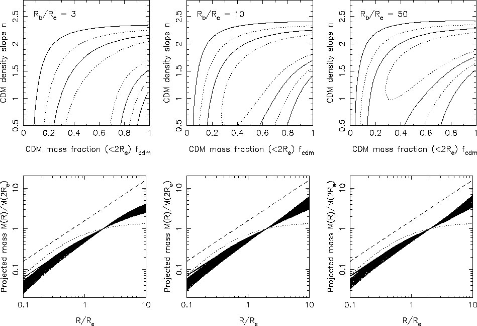Figure B.32. The structure of lens galaxies in self-similar models. The top row shows the permitted region for the slope of the inner dark matter cusp ( r-n) and the projected fraction of the mass fCDM inside 2Re composed of dark matter. The results are shown for three ratios Rb / Re between the break radius Rb of the dark matter profile and the effective radius Re of the luminous galaxy. The solid (dashed) contours show the 68% and 95% confidence levels for two (one) parameter. Note that the estimates of n and fCDM depend little on the location of the break radius relative to the effective radius. The bottom row shows all the mass profiles lying within the (two parameter) 68% confidence region normalized to a fixed projected mass inside 2Re. For comparison we show the mass enclosed by a de Vaucouleurs model (dotted line) and an SIS (offset dashed line). While the allowed models exhibit a wide range of dark matter abundances, slopes and break radii, they all have roughly isothermal total mass profiles over the radial range spanned by the lensed images.

⁴ They could also have allowed the CDM fraction to vary as f_CDM L^y, but these led to degenerate models where only the combination x + y was constrained. Back.