6. AXIONS

6.1. "Invisible" axions

Axions are hypothetical particles whose existence would explain what is otherwise a puzzling feature of quantum chromodynamics (QCD), the leading theory of strong interactions. QCD contains a dimensionless free parameter () whose value must be "unnaturally" small in order for the theory not to violate a combination of charge conservation and mirror-symmetry known as charge parity or CP. Upper limits on the electric dipole moment of the neutron currently constrain the value of to be less than about 10^-9. The strong CP problem is the question: "Why is so small?" This is reminiscent of the cosmological-constant problem (Sec. 4.5), though less severe by many orders of magnitude. Proposed solutions have similarly focused on making , like , a dynamical variable whose value could have been driven toward zero in the early Universe. In the most widely-accepted scenario, due to Peccei and Quinn in 1977 [204], this is accomplished by the spontaneous breaking of a new global symmetry (now called PQ symmetry) at energy scales f_PQ. As shown by Weinberg [205] and Wilczek [206] in 1978, the symmetry-breaking gives rise to a new particle which eventually acquires a rest energy m_a c² f_PQ^-1. This particle is the axion (a).

Axions, if they exist, meet all the requirements of a successful CDM candidate (Sec. 4.3): they interact weakly with the baryons, leptons and photons of the standard model; they are cold (i.e. non-relativistic during the time when structure begins to form); and they are capable of providing some or even all of the CDM density which is thought to be required, _cdm ~ 0.3. A fourth property, and the one which is of most interest to us here, is that axions decay generically into photon pairs. The importance of this process depends on two things: the axion's rest mass m_a and its coupling strength g_a. The PQ symmetry-breaking energy scale f_PQ is not constrained by the theory, and reasonable values for this parameter are such that m_a c² might in principle lie anywhere between 10^-12 eV and 1 MeV [96]. This broad range of theoretical possibilities has been whittled down by an impressive array of cosmological, astrophysical and laboratory-based tests. In summarizing these, it is useful to distinguish between axions with rest energies above and below a "critical" rest energy m_{a, crit} c² ~ 3 × 10^-2 eV.

Axions whose rest energies lie below m_{a, crit}c² arise primarily via processes known as vacuum misalignment [207, 208, 209] and axionic string decay [210]. These are non-thermal mechanisms, meaning that the axions produced in this way were never in thermal equilibrium with the primordial plasma. Their present density would be at least [211]

(163)

(This number is currently under debate, and may go up by an order of magnitude or more if string effects play an important role [212].) If we require that axions not provide too much CDM (_cdm 0.6) then (163) implies a lower limit on the axion rest energy:

(164)

This neatly eliminates the lower third of the theoretical axion mass window. Upper limits on m_a for non-thermal axions have come from astrophysics. Prime among these is the fact that the weak couplings of axions to baryons, leptons and photons allow them to stream freely from stellar cores, carrying energy with them. If they are massive enough, such axions could in principle cool the core of the Sun, alter the helium-burning phase in red-giant stars, and shorten the duration of the neutrino burst from supernovae such as SN1987a. The last of these effects is particularly sensitive and requires [213, 214]:

(165)

Axions with 10^-5 m_a c² 10^-2 thus remain compatible with both cosmological and astrophysical limits, and could provide much or all of the CDM. It may be possible to detect these particles in the laboratory by enhancing their conversion into photons with strong magnetic fields, as demonstrated by Sikivie in 1983 [215]. Experimental search programs based on this principle are now in operation at the Lawrence Livermore lab in the U.S.A. [216], Tokyo [217], the Sierra Grande mountains in Argentina (SOLAX [218]), the Spanish Pyrenees (COSME [219]) and CERN in Switzerland (CAST [220]). Exclusion plots from these experiments are beginning to restrict theoretically-favoured regions of the phase space defined by m_a and g_a.

Promising as they are, we will not consider non-thermal axions (sometimes known as "invisible axions") further in this section. This is because they decay too slowly to leave any trace in the extragalactic background light. Axions decay into photon pairs (a + ) via a loop diagram, as illustrated in Fig. 24. The decay lifetime of this process is [96]

(166)

Here m₁ m_ac² / (1 eV) is the axion rest energy in units of eV, and is a constant which is proportional to the coupling strength g_a [221]. For our purposes, it is sufficient to treat as a free parameter which depends on the details of the axion theory chosen. Its value has been normalized in Eq. (166) so that = 1 in the simplest grand unified theories (GUTs) of strong and electroweak interactions. This could drop to = 0.07 in other theories, however [222], strongly suppressing the two-photon decay channel. In principle could even vanish altogether, corresponding to a radiatively stable axion, although this would require an unlikely cancellation of terms. We will consider values in the range 0.07 1 in what follows. For these values of , and with m₁ 6 × 10^-3 as given by (165), Eq. (166) shows that axions decay on timescales _a 9 × 10³⁵ s. This is so much longer than the age of the Universe that such particles would truly be invisible.

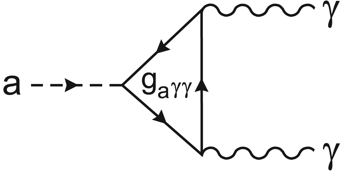Figure 24. The Feynman diagram corresponding to the decay of the axion (a) into two photons () with coupling strength ga.

6.2. The multi-eV window

We therefore shift our attention to axions with rest energies above m_{a, crit} c². Turner showed in 1987 [223] that the vast majority of these would have arisen in the early Universe via thermal mechanisms such as Primakoff scattering and photo-production. The Boltzmann equation can be solved to give their present comoving number density as n_a = (830 / g_*F) cm^-3 [221], where g_*F 15 counts the number of relativistic degrees of freedom left in the plasma at the time when axions "froze out" of equilibrium. The present density parameter _a = n_a m_a / _crit,0 of thermal axions is thus

(167)

Whether or not this is significant depends on the axion rest mass. The duration of the neutrino burst from SN1987a again imposes a powerful constraint on m_a c². This time, however, it is a lower, not an upper bound, because axions in this range of rest energies are massive enough to interact with nucleons in the supernova core and can no longer stream out freely. Instead, they are trapped in the core and radiate only from an "axiosphere" rather than the entire volume of the star. Axions with sufficiently large m_a c² are trapped so strongly that they no longer interfere with the luminosity of the neutrino burst, leading to the lower limit [224]

(168)

Astrophysics also provides strong upper bounds on m_a c² for thermal axions. These depend critically on whether or not axions couple only to hadrons, or to other particles as well. An early class of hadronic axions (those coupled only to hadrons) was developed by Kim [225] and Shifman, Vainshtein and Zakharov [226]; these particles are often termed KSVZ axions. Another widely-discussed model in which axions couple to charged leptons as well as nucleons and photons has been discussed by Zhitnitsky [227] and Dine, Fischler and Srednicki [228]; these particles are known as DFSZ axions. The extra lepton coupling of these DFSZ axions allows them to carry so much energy out of the cores of red-giant stars that helium ignition is seriously disrupted unless m_a c² 9 × 10^-3 eV [229]. Since this upper limit is inconsistent with the lower limit (168), thermal DFSZ axions are excluded. For KSVZ or hadronic axions, red giants impose a weaker bound [230]:

(169)

This is consistent with the lower limit (168) for realistic values of the parameter . For the simplest hadronic axion models with 0.07, for instance, Eq. (169) translates into an upper limit m_a c² 10 eV. It has been argued that axions with m_a c² 10 eV can be ruled out in any case because they would interact strongly enough with baryons to produce a detectable signal in existing Cerenkov detectors [231].

For thermally-produced hadronic axions, then, there remains a window of opportunity in the multi-eV range with 2 m₁ 10. Eq. (167) shows that these particles would contribute a total density of about 0.03 _a 0.15, where we take 0.6 h₀ 0.9 as usual. They would not be able to provide the entire density of dark matter in the CDM model (_m,0 = 0.3), but they could suffice in low-density models midway between CDM and BDM (Table 2). Since such models remain compatible with most current observational data (Sec. 4), it is worth proceeding to see how these multi-eV axions can be further constrained by their contributions to the EBL.

6.3. Axion halos

Thermal axions are not as cold as their non-thermal cousins, but will still be found primarily inside gravitational potential wells such as those of galaxies and galaxy clusters [223]. We need not be too specific about the fraction which have settled into galaxies as opposed to larger systems, because we will be concerned primarily with their combined contributions to the diffuse background. (Distribution could become an issue if extinction due to dust or gas played a strong role inside the bound regions, but this is not likely to be important for the photon energies under consideration here.) These axion halos provide us with a convenient starting-point as cosmological light sources, analogous to the galaxies and vacuum source regions of previous sections. Let us take the axions to be cold enough that their fractional contribution (M_h) to the total mass of each halo (M_tot) is the same as their fractional contribution to the cosmological matter density, M_h / M_tot = _a / _m,0 = _a / (_a + _bar). Then the mass M_h of axions in each halo is

(170)

(Here we have made the minimal assumption that axions constitute all the nonbaryonic dark matter.) If these halos are distributed with a mean comoving number density n₀, then the cosmological density of bound axions is _a,bound = (n₀ M_h) / _crit,0 = (n₀ M_tot / _crit,0)(1 + _bar / _a)^-1. Equating _a,bound to _a, as given by (167), fixes the total mass:

(171)

The comoving number density of galaxies at z = 0 is [200]

(172)

Using this together with (167) for _a, and setting _bar 0.016h₀^-2 from Sec. 4.2, we find from (171) that

(173)

Let us compare these numbers with dynamical data on the mass of the Milky Way using the motions of Galactic satellites. These assume a Jaffe profile [232] for halo density:

(174)

where v_c is the circular velocity, r_j the Jaffe radius, and r the radial distance from the center of the Galaxy. The data imply that v_c = 220 ± 30 km s^-1 and r_j = 180 ± 60 kpc [75]. Integrating over r from zero to infinity gives

(175)

This is consistent with (173) for most values of m₁ and h₀. So axions of this type could in principle make up all the dark matter which is required on Galactic scales.

Putting (171) into (170) gives the mass of the axion halos as

(176)

This could also have been derived as the mass of a region of space of comoving volume V₀ = n₀^-1 filled with homogeneously-distributed axions of mean density _a = _{a crit,0}. (This is the approach that we adopted in defining vacuum regions in Sec. 5.6.)

To obtain the halo luminosity, we sum up the rest energies of all the decaying axions in the halo and divide by the decay lifetime (166):

(177)

Inserting Eqs. (166) and (176), we find

			(178)

The luminosities of the galaxies themselves are of order L₀ = ₀ / n₀ = 2 × 10¹⁰ h₀^-2 L, where we have used (20) for ₀. Thus axion halos could in principle outshine their host galaxies, unless axions are either very light (m₁ 3) or weakly-coupled ( < 1). This already suggests that they will be strongly constrained by observations of EBL intensity.

6.4. Bolometric intensity

Substituting the halo comoving number density (172) and luminosity (178) into Eq. (15), we find that the combined intensity of decaying axions at all wavelengths is given by

(179)

Here the dimensional content of the integral is contained in the prefactor Q_a, which takes the following numerical values:

			(180)

There are three things to note about this quantity. First, it is comparable in magnitude to the observed EBL due to galaxies, Q_* 3 × 10^-4 erg s^-1 cm^-2 (Sec. 2). Second, unlike Q_* for galaxies or Q_v for decaying vacuum energy, Q_a depends explicitly on the uncertainty h₀ in Hubble's constant. Physically, this reflects the fact that the axion density _a = _{a crit,0} in the numerator of (180) comes to us from the Boltzmann equation and is independent of h₀, whereas the density of luminous matter such as that in galaxies is inferred from its luminosity density ₀ (which is proportional to h₀, thus cancelling the h₀-dependence in H₀). The third thing to note about Q_a is that it is independent of n₀. This is because the collective contribution of decaying axions to the diffuse background is determined by their mean density _a, and does not depend on how they are distributed in space.

To evaluate (179) we need to specify the cosmological model. If we assume a spatially flat Universe, as increasingly suggested by the data (Sec. 4), then Hubble's parameter (33) reads

(181)

where we take the most economical approach and require axions to make up all the cold dark matter so that _m,0 = _a + _bar. Putting this into Eq. (179) along with (180) for Q_a, we obtain the plots of Q(m₁) shown in Fig. 25 for = 1. The three heavy lines in this plot show the range of intensities obtained by varying h₀ and _bar h₀² within the ranges 0.6 h₀ 0.9 and 0.011 _bar h₀² 0.021 respectively. We have set z_f = 30, since axions were presumably decaying long before they became bound to galaxies. (Results are insensitive to this choice, rising by less than 2% as z_f 1000 and dropping by less than 1% for z_f = 6.) The axion-decay background is faintest for the largest values of h₀, as expected from the fact that Q_a h₀^-1. This is partly offset by the fact that larger values of h₀ also lead to a drop in _m,0, extending the age of the Universe and hence the length of time over which axions have been contributing to the background. (Smaller values of _bar raise the intensity slightly for the same reason.) Fig. 25 shows that axions with = 1 and m_a c² 3.5 eV produce a background brighter than that from the galaxies themselves.

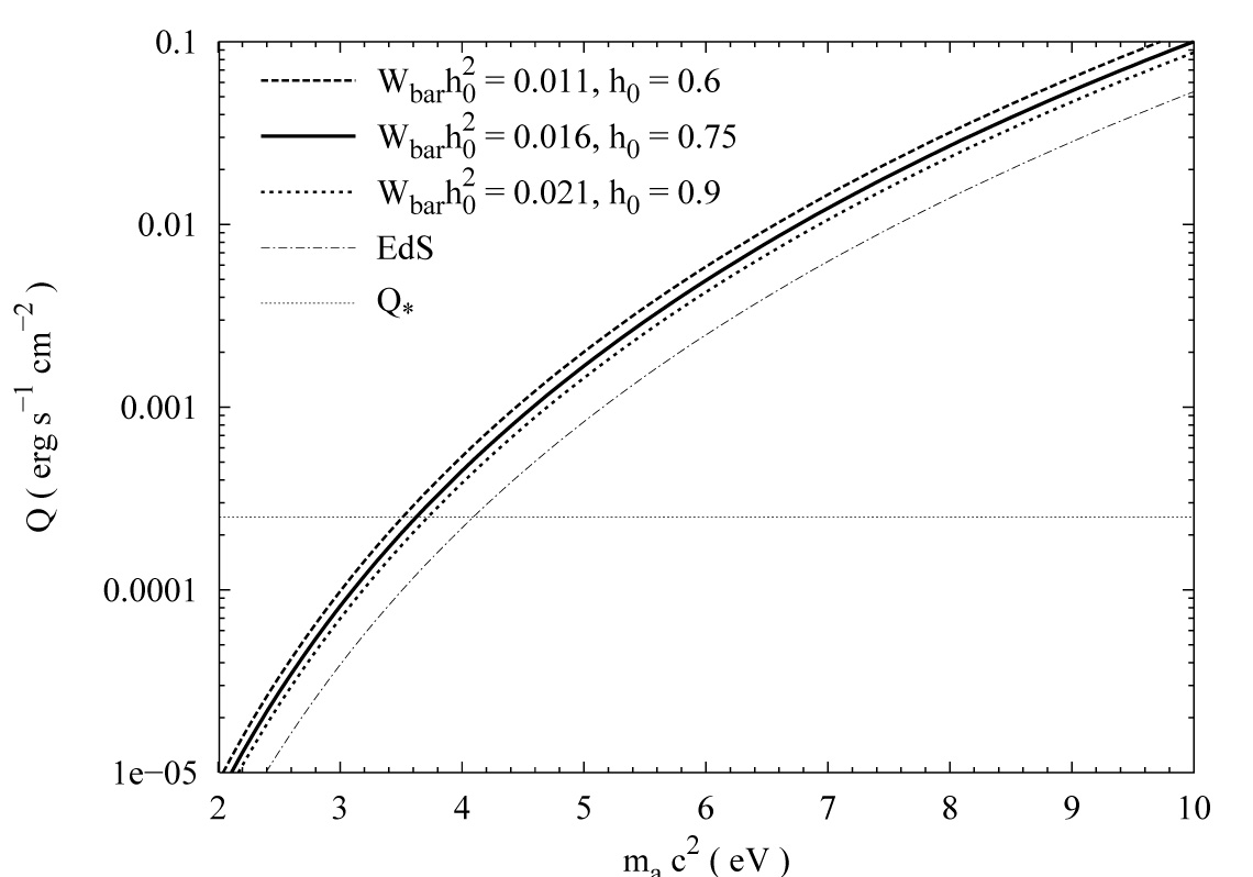Figure 25. The bolometric intensity Q of the background radiation from decaying axions as a function of their rest masses ma. The faint dash-dotted line shows the equivalent intensity in an EdS model (in which axions alone cannot provide the required CDM). The dotted horizontal line indicates the characteristic bolometric intensity (Q*) of the observed EBL.

6.5. The infrared and optical backgrounds

To go further and compare our predictions with observational data, we would like to calculate the intensity of axionic contributions to the EBL as a function of wavelength. The first step, as usual, is to specify the spectral energy distribution or SED of the decay photons in the rest frame. Each axion decays into two photons of energy 1/2 m_a c² (Fig. 24), so that the decay photons are emitted at or near a peak wavelength

(182)

Since 2 m₁ 10, the value of this parameter tells us that we will be most interested in the infrared and optical bands (roughly 4000-40,000 Å). We can model the decay spectrum with a Gaussian SED as in (75):

(183)

For the standard deviation of the curve, we can use the velocity dispersion v_c of the bound axions [234]. This is 220 km s^-1 for the Milky Way, implying that 40 Å / m₁ where we have used = 2(v_c / c) _a (Sec. 3.4). For axions bound in galaxy clusters, v_c rises to as much as 1300 km s^-1 [221], implying that 220 Å / m₁. Let us parametrize in terms of a dimensionless quantity ₅₀ / (50 Å / m₁) so that

(184)

With the SED F() thus specified along with Hubble's parameter (181), the spectral intensity of the background radiation produced by axion decays is given by (62) as

(185)

The dimensional prefactor in this case reads

			(186)

We have divided through by the photon energy hc / ₀ to put results into continuum units or CUs as usual (Sec. 3.2). The number density in (62) cancels out the factor of 1 / n₀ in luminosity (178) so that results are independent of axion distribution, as expected. Evaluating Eq. (185) over 2000 Å ₀ 20,000 Å with = 1 and z_f = 30, we obtain the plots of I(₀) shown in Fig. 26. Three groups of curves are shown, corresponding to m_a c² = 3 eV, 5 eV and 8 eV. For each value of m_a there are four curves; these assume (h₀, _bar h₀²) = (0.6, 0.011),(0.75, 0.016) and (0.9, 0.021) respectively, with the fourth (faint dash-dotted) curve representing the equivalent intensity in an EdS universe (as in Fig. 25). Also plotted are many of the reported observational constraints on EBL intensity in this waveband. Most have been encountered already in Sec. 3. They include data from the OAO-2 satellite (LW76 [20]), several ground-based telescope observations (SS78 [21], D79 [22], BK86 [23]), the Pioneer 10 spacecraft (T83 [18]), sounding rockets (J84 [24], T88 [25]), the Space Shuttle-borne Hopkins UVX experiment (M90 [26]), the DIRBE instrument aboard the COBE satellite (H98 [27], WR00 [28], C01 [29]), and combined HST/Las Campanas telescope observations (B02 [30]).

Figure 26. The spectral intensity I of the background radiation from decaying axions as a function of observed wavelength 0. The four curves for each value of ma (labelled) correspond to upper, median and lower limits on h0 and bar together with the equivalent intensity for the EdS model (as in Fig. 25). Also shown are observational upper limits (solid symbols and heavy lines) and reported detections (empty symbols) over this waveband.

Fig. 26 shows that 8 eV axions with = 1 would produce a hundred times more background light at ~ 3000 Å than is actually seen. The background from 5 eV axions would similarly exceed observed levels by a factor of ten at ~ 5000 Å, colouring the night sky green. Only axions with m_a c² 3 eV are compatible with observation if = 1. These results are brighter than ones obtained assuming an EdS cosmology [233], especially at wavelengths longward of the peak. This reflects the fact that the background in a low-_m,0, high-_,0 universe like that considered here receives many more contributions from sources at high redshift.

To obtain more detailed constraints, we can instruct a computer to evaluate the integral (185) at more finely-spaced intervals in m_a. Since I ^-2, the value of required to reduce the minimum predicted axion intensity I_th below a given observational upper limit I_obs at any wavelength ₀ in Fig. 26 is (I_obs / I_th)^1/2. The upper limit on (for a given value of m_a) is then the smallest such value of ; i.e. that which brings I_th down to I_obs or below at each wavelength ₀. From this procedure we obtain a function which can be regarded as an upper limit on the axion rest mass m_a as a function of (or vice versa). Results are plotted in Fig. 27 (heavy solid line). This curve tells us that even in models where the axion-photon is strongly suppressed and = 0.07, the axion cannot be more massive than

(187)

In the simplest axion models with = 1, this limit tightens to

(188)

As expected, these bounds are stronger than those obtained in an EdS model, for which some other CDM candidate would have to be postulated besides the axions (Fig. 27, faint dotted line). This is a small effect, however, because the strongest constraints tend to come from the region near the peak wavelength (_a), whereas the difference between matter- and vacuum-dominated models is most pronounced at wavelengths longward of the peak where the majority of the radiation originates at high redshift. Fig. 27 shows that cosmology in this case has the most effect over the range 0.1 0.4, where upper limits on m_a c² are weakened by about 10% in the EdS model relative to one in which the CDM is assumed to consist only of axions.

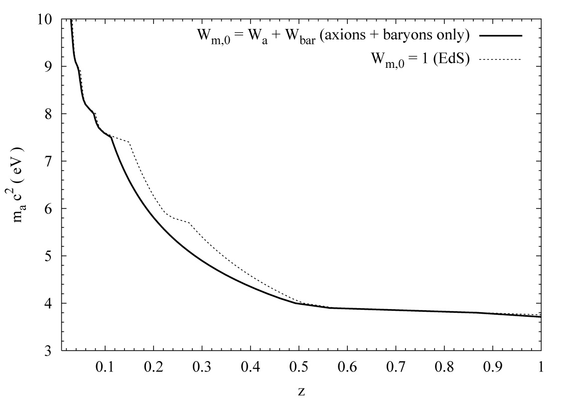Figure 27. The upper limits on the value of ma c2 as a function of the coupling strength (or vice versa). These are derived by requiring that the minimum predicted axion intensity (as plotted in Fig. 26) be less than or equal to the observational upper limits on the intensity of the EBL.

Combining Eqs. (168) and (188), we conclude that axions in the simplest models are confined to a slender range of viable rest masses:

(189)

Background radiation thus complements the red-giant bound (169) and closes off most, if not all of the multi-eV window for thermal axions. The range of values (189) can be further narrowed by looking for the enhanced signal which might be expected to emanate from concentrations of bound axions associated with galaxies and clusters of galaxies, as first suggested by Kephart and Weiler in 1987 [234]. The most thorough search along these lines was reported in 1991 by Bershady [235], who found no evidence of the expected signal from three selected clusters, further tightening the upper limit on the multi-eV axion window to 3.2 eV in the simplest models. Constraints obtained in this way for non-thermal axions would be considerably weaker, as noticed by several workers [234, 236], but this does not affect our results since axions in the range of rest masses considered here are overwhelmingly thermal ones. Similarly, "invisible" axions with rest masses near the upper limit given by Eq. (165) might give rise to detectable microwave signals from nearby mass concentrations such as the Local Group of galaxies; this is the premise for a recent search carried out by Blout [237] which yielded an independent lower limit on the coupling parameter g_a.

Let us turn finally to the question of how much dark matter can be provided by light thermal axions of the type we have considered here. With rest energies given by (189), Eq. (167) shows that

(190)

Here we have taken 0.6 h₀ 0.9 as usual. This is comparable to the density of baryonic matter (Sec. 4.2), but falls well short of most expectations for the density of cold dark matter.

Our main conclusions, then, are as follows: thermal axions in the multi-eV window remain (only just) viable at the lightest end of the range of possible rest-masses given by Eq. (189). They may also exist with slightly higher rest-masses, up to the limit given by Eq. (187), but only in certain axion theories where their couplings to photons are weak. In either of these two scenarios, however, their contributions to the density of dark matter in the Universe are so feeble as to remove much of their motivation as CDM candidates. If they are to provide a significant portion of the dark matter, then axions must have rest masses in the "invisible" range where they do not contribute significantly to the light of the night sky.