4. BEYOND THE SIMPLEST MODELS OF THE GALAXY–HALO CONNECTION

The simplest versions of the empirical models we outlined in Section 2, which connect one primary galaxy property to one halo property, describe the basic relations very well. However, they have now been shown in the literature to be inadequate for describing both the spatial distribution of galaxies at the precision it can now be measured and the full richness of galaxy properties and correlations that are observable. Here, we discuss additional modeling aspects that may be required. We first discuss the question of which halo property should be primary (Section 4.1). We then consider the question of alternative primary galaxy properties (Section 4.2). We then review other aspects of the galaxy–halo connection that can impact clustering properties, even for a given SHMR: scatter between galaxy mass and halo mass (Section 4.3), assembly bias (Section 4.4), and the ratio of galaxy mass to halo mass between centrals and satellites (or, equivalently, the satellite fraction as a function of stellar mass; Section 4.5). We then discuss properties of the satellite distribution (Section 4.6), and consider approaches to joint modeling of additional galaxy properties, including galaxy star formation rates, galaxy sizes, and gas properties.

4.1. What halo property is best matched to galaxies?

The existence of a galaxy–halo connection does not specify which galaxy property correlates with which halo property, though mass is a typical assumption for both. Mapping galaxy stellar mass to different halo properties will yield the same SMF, but different clustering signals. Kravtsov et al. (2004) originally proposed using the maximum circular velocity of halos V_max — both parent halos and subhalos — to match onto galaxies. Whereas the mass of a subhalo is subject to intense tidal stripping immediately upon entering a larger halo, V_max is more robust to stripping. A solution to the tidal stripping problem that allows one to use M_h is to use M_h at the time the subhalo was accreted in order to match to galaxy properties. These ideas can be combined in various ways, all of which yield slightly different results in terms of the spatial distribution of galaxies.

Different Halo Properties for Abundance Matching

• M₀: The halo mass today or at the epoch being modeled.
• M_acc: Mass at the time of accretion. Equivalent to M₀ for host halos.
• M_peak: In the entire history of a halo, the highest mass achieved.
• V₀. Maximum circular velocity of the halo today or at the epoch being modeled.
• V_acc: The V_max at the time of accretion. Equivalent to V_max for host halos.
• V_peak: In the entire history of a halo, the highest V_max achieved.
• M_0,peak and V_0,peak: For subhalos, M_peak or V_peak. For host halos, these values are taken at the epoch being modeled.
• V^α: a smooth transition between M_peak and V_peak: v_vir(v_max / v_vir)^α, with 0 ≤ α ≤ 1.

Each of the halo properties in the sidebar titled Different Halo Properties for Abundance Matching can be used, either in a non-parametric abundance matching model or in a parameterized SHMR, to map galaxies onto halos to match the observed luminosity function or SMF. Each of these models will produce slightly different spatial distributions, quantified by the two-point correlation functions shown in Figure 4. In general, the models that use V_max, in some form or another, produce galaxy samples that are more highly clustered than models that use M_h. This is due to two effects which can both impact the clustering: assembly bias, and the different relationships between the properties of centrals and satellites. We discuss the former in Section 4.4. For the latter, the impact of different abundance matching quantities is clearly seen in the right-hand side of Figure 4, which shows the satellite fraction, f_sat, for each of the models as a function of galaxy stellar mass. Models with a higher f_sat yield a higher clustering amplitude, especially at smaller scales (r_p < 1 Mpc).

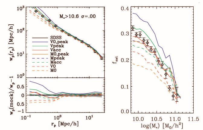Figure 4. Left Panel: Projected galaxy clustering as a function of scale, for different variants of abundance matching models, where the galaxy properties are matched to different halo properties. In these models no scatter is assumed. Points with error bars are measurements from SDSS. Right Panel: The fraction of galaxies that are satellites as a function of M∗. The line types are the same as in the left panel. Points with error bars are from the SDSS galaxy group catalog of Tinker, Wetzel & Conroy (2011). All theoretical models have been passed through the group finder to account for any biases in this process. Both panels are from Reddick et al. (2013).

4.2. What galaxy property is best matched to halos?

Through most of this review, we consider galaxy stellar mass to be the primary galaxy property that is most tightly correlated with the properties of the galaxy halos. However, it is interesting to consider other possibilities. In the literature, galaxy stellar mass and galaxy luminosity have been treated rather interchangeably. It is likely that observational uncertainties in measuring galaxy masses and luminosities may be larger than the difference in the scatter between them, but with higher precision measurements it may be possible to make this distinction. The total stellar mass or luminosity in groups and clusters of galaxies is better correlated with halo mass than is the stellar mass or luminosity of the central galaxy; the former scales roughly as M_∗,tot ∼ M_h^2/3 on the massive end, whereas the latter scales roughly as M_∗,cen ∼ M_h^1/3 on the massive end (e.g. Lin & Mohr, 2004).

Most of this review assumes that stars in galaxies are setting the primary property, instead of gas. This is largely due to the fact that obtaining large complete samples of galaxies with consistently measured gas properties is very challenging. A first basic question is whether the correlation between halo mass and total baryon mass is stronger than the correlation with stellar mass. This has been studied extensively with the Tully-Fisher relationship (e.g., McGaugh et al. 2000), and also with clustering of HI-selected samples (e.g., Guo et al. 2017). At the current level of accuracy, the scatter between stellar mass–halo mass and baryon mass–halo mass appear to be comparable, although this may be more likely to break down for smaller mass galaxies which have high gas fractions (Bradford, Geha & Blanton, 2015). Future large HI surveys should allow a more comprehensive study of this question.

An alternative galaxy property is galaxy size. Accurate statistical modeling is becoming especially interesting now that the relationship between galaxy sizes and stellar masses have been measured for larger samples in the local Universe (Cappellari et al., 2013) and over a wide range of epochs with HST (van der Wel et al., 2014). Despite the complexity of galaxy formation, the tight scaling relations observed between various galaxy structural parameters imply a fairly tight connection between galaxy sizes and the properties of their dark matter halos. We discuss joint modeling of two galaxy properties further in Section 4.7.

4.3. Scatter

One of the principle questions about the galaxy–halo connection is how much scatter there is between the properties of galaxies at a given halo mass. When comparing models, we consider scatter in the SHMR of central galaxies, e.g. the scatter in M_∗ at fixed M_h, which we refer to as σ_{log M∗}. In abundance matching models the actual parameterization is in terms of the matching proxy (see the sidebar titled Different Halo Properties for Abundance Matching), and this scatter is generally assumed to be lognormal and constant across all halo masses. This is both for convenience and because these assumptions appear to be consistent with all present data, including the results for fitting HOD models to galaxy threshold samples. See, for example, Behroozi, Conroy & Wechsler (2010) for the methodology of incorporating scatter in abundance matching while preserving the same stellar mass function.

HOD models parameterize the mean number of galaxies per halo. For HOD models of luminosity or stellar mass threshold samples, the scatter is incorporated in the shape of the central galaxy occupation function. For central galaxies, because there can only be one or zero centrals, this translates to the probability of having a galaxy above the threshold as a function of halo mass. Thus the scatter derived in HOD models of this type is related to (but not exactly) the scatter in halo mass at a fixed galaxy mass (or luminosity). The HOD analysis of SDSS galaxies by Zehavi et al. (2011) found that this scatter — the scatter in M_h at fixed L_gal — monotonically rises with increasing L_gal.

Figure 5 (left panel) shows the full two-dimensional distribution of halo masses and galaxy masses for the fiducial model that matches the stellar mass function and clustering of SDSS galaxies presented in Figure 3. One can see that in such a model the scatter in M_h at fixed M_∗ will depend sensitively on the value of M_∗ itself. The middle panel shows σ(M_h | M_∗) explicitly. Above the pivot point the mean relation between M_∗ and M_h is shallower, and galaxies across a fixed width in logM_∗ are spread out over a wider range of logM_h.

Figure 5. Left Panel: The full distribution of halo and galaxy stellar masses for the abundance matching model from Figure 3 (i.e., the orange curve in that Figure). Both halos and subhalos are included. The gray scale indicates the log of the number of objects in each bin in the two-dimensional plane. In this model, the scatter of stellar mass at fixed halo mass is constant, with σlog M∗ = 0.2 dex. The red dashed lines show the inner 68% range of M∗ at fixed Mh, which is 0.4 dex across the y-axis. However, due to the change in the slope of the SHMR at Mh > 1012 M⊙, the distribution in Mh at fixed M∗ widens considerably above this mass. Middle Panel: The scatter in Mh at fixed M∗, σ(Mh | M∗) for the model in the left-hand panel. At low masses, this scatter is a constant value equal to roughly half of σlog M∗. Above the pivot point in the SHMR, the scatter monotonically increases, due both to the change in slope in the SHMR and to the changing slope of the halo mass function, which exponentially declines at high Mh. Right Panel: The solid curves show three different fits to the SDSS stellar mass function in Figure 3, all with different values of σlog M∗. These solid curves all show the SHMR as the mean value of M∗ in bins of Mh. The dashed curves show the corresponding reverse relationship, the mean value of Mh in bins of M∗. As σlog M∗ increases, the mean halo mass at fixed M∗ decreases, even though the mean M∗ at fixed Mh decreases with increasing σlog M∗.

In abundance matching models, various choices for σ_{log M∗} can yield the same stellar mass function, but they do not predict the same spatial distribution of galaxies. The right-hand panel of Figure 5 shows three different SHMRs, all three of which provide good fits to the same SDSS stellar mass function but have three different values of σ_{log M∗}. The solid curves show each SHMR as the mean M_∗ as a function of M_h. As σ_{log M∗} increases, the solid curves decrease at fixed M_h. In other words, the halo mass that yields a mean galaxy mass of ⟨ M_∗⟩ = 10^11.5 M_⊙ increases with σ_{log M∗}. But recall that each model produces the same abundance of galaxies. Higher mass halos are less abundant, but the larger scatter brings in more low-mass halos that contain 10^11.5 M_⊙ galaxies to preserve the same abundance. This has a direct impact on the clustering of galaxies, as higher mass halos above M_h > 10¹² M_⊙ become increasingly more clustered (more highly biased). Thus the highest sensitivity to σ_{log M∗} from clustering measurements is in samples of galaxies at high masses or luminosities.

4.4. Assembly bias

Halos and galaxies experience a wide variety of assembly histories, even at fixed masses. Different assembly histories can influence the secondary properties of halos and galaxies. Assembly history also correlates with large-scale environment, yielding a correlation between some secondary properties and the spatial distribution of objects. In this subsection, we review how this assembly bias manifests for halos, and how this might propagate into the galaxy population.

4.4.1. Halo assembly bias.   Halo assembly bias refers to the effect that the clustering of halos at fixed mass has a dependence on properties other than M_h. This dependence was initially detected when sorting halos at a given mass by formation time, concentration, and spin (Wechsler, 2001, Gao, Springel & White, 2005, Wechsler et al., 2006), as well as for simulated galaxy samples (Croton, Gao & White, 2007), and has now been studied extensively in the literature for a number of properties of dark matter halos (see, e.g., Mao, Zentner & Wechsler (2018) for a recent comprehensive study). Figure 6 shows an example of halo assembly bias that can be seen visually in the distribution of low-mass halos, as well as a quantitative assessment. Different assembly bias effects can be created from tidal forces in the density field (Hahn et al. 2009), and from the statistics of peaks in a Gaussian random field (Dalal et al. 2008).

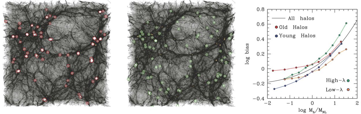Figure 6. Halo assembly bias, manifesting in concentration, halo formation time, and halo angular momentum. Left Panel: The gray scale shows the distribution of dark matter in a 90 x 90 x 30 Mpc slice of a cosmological simulation at z = 0. The open red circles indicate the 5% of halos at logMh = 10.8 with the highest concentration. Middle Panel: The same slice is shown once again, but here the green circles show the locations of the 5% of halos with the lowest concentration from the same halo mass range. Right Panel: The dependence of halo bias on secondary parameters. Bias here refers to clustering amplitude relative to dark matter, as defined in Section 3.2. The solid black curve shows the overall bias of dark matter halos as a function of halo mass at z = 0. The red and blue points show the clustering for the 25% of halos with the highest formation redshift and lowest formation redshift, respectively. Data are taken from Li, Mo & Gao (2008). The orange and green points show the clustering for the 20% of halos with the highest and lowest angular momentum, respectively. Data are taken from Bett et al. (2007).

Although its existence for dark matter halos is now well established, there are many open questions about the assembly bias signal for various halo properties and whether or to what extent this effect propagates into the clustering of galaxies. We summarize some of these properties in the sidebar titled What Halo Properties Show Secondary Bias?, but note that in general, the secondary bias of various halo properties can be complex, and can have different mass and redshift dependence (Salcedo et al., 2018). Furthermore, Mao, Zentner & Wechsler (2018) have shown that even properties that are highly correlated do not necessarily have the same clustering signal. This may make first principles predictions for the expected galaxy assembly bias challenging, but it also indicates that precision measurements of galaxy clustering may provide insights into complex details of structure formation and the dependence of galaxy properties on halo properties.

Important Definitions

• Bias: The clustering of a set of objects relative to the clustering of dark matter.
• Halo Assembly Bias or Secondary Bias: At fixed halo mass, the clustering of dark matter halos depends on secondary halo properties (which are generally correlated with the assembly history of the dark matter halo).
• Galaxy Assembly Bias: At fixed halo mass, the galaxy properties or number of galaxies within dark matter halos may depend on secondary halo properties that themselves show a halo assembly bias signature. This includes both central and satellite galaxies. Note that this definition, proposed by Zentner, Hearin & van den Bosch (2014) is not exactly parallel with the definition of halo assembly bias definition, and is dependent on the existence of halo assembly bias. It is well known that galaxy clustering depends on secondary galaxy properties, but this can be caused by different satellite fractions or a dependence on halo mass for the secondary property.

What halo properties show secondary bias?

• Halo properties that show stronger assembly bias at lower masses: half-mass redshift z_M/2, formation redshift a_c, fractional halo growth rate ΔM / M. These quantities are usually defined with respect to M_h at z = 0, but they show assembly bias when defined at any redshift.
• Halo properties that show stronger assembly bias at higher masses: angular momentum λ, amount of substructure.
• Halo concentration shows signals at high and low masses, but the sign of the signal switches at the non-linear halo mass M ∼ M_NL.

4.4.2. Theoretical models of galaxy assembly bias   In the abundance matching paradigm, the relation between galaxies and halos is set by the halo property that is used to match to the given galaxy property. However, there is no a priori reason to limit the model to a single halo property. In the literature, there have been multiple models for multi-parameter galaxy–halo connections. Here we list two that vary the galaxy clustering properties for luminosity or mass selected galaxy samples; models that include assembly bias for secondary properties like color or star formation rate are discussed in Section 4.7.

Composite abundance matching: In this model, the abundance matching parameter is a combination of two or more halo properties. In the model by Lehmann et al. (2017), the abundance matching parameter is

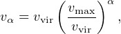(1)

where v_vir = (GM_vir / R_vir)^1/2 is the virial velocity of the halo, and v_max is the maximum circular velocity within the halo, and α is a free parameter. When α = 0, the abundance matching parameter is v_vir, which is directly proportional to M_vir^1/3 — i.e., abundance matching galaxy mass to halo mass. When α = 1, the abundance matching parameter is v_max, which is directly related to halo concentration. This process is implemented on halo catalogs that resolve substructure. In Lehmann et al. (2017) these halo quantities are evaluated at the epoch of peak halo mass. Increasing α, therefore, has the effect of increasing the clustering at fixed M_∗ (because of the effect of concentration on clustering, as shown in Figure 6). This freedom essentially parameterizes our current ignorance about how much galaxy properties depend on concentration or formation time at a given halo mass, which impacts both the assembly bias and the satellite fraction at a given stellar mass.

Modified halo occupation models: The previous approach requires simulations that resolve substructure. An alternative is to take parameterized HOD models — i.e., models in which the mean occupation function of central and satellite galaxies are parameterized as a function of M_h — and modify them to include additional halo properties in the mean occupation function. These models require cosmological simulations or a multi-parameter emulator based on such simulations, but no longer require that substructure be tracked. Hearin et al. (2016) proposed decorated HODs, with the secondary parameter being halo concentration; Tinker et al. (2008a) used large-scale density as the secondary parameter to make models to compare to measurements of clustering and voids. In the decorated HOD models, the mean occupation function is increased or decreased, relative to the mean at a given value of M_h, on the basis of whether the concentration is above or below the median c. The change in the HOD can be either a step function or a smooth function in c, and can be either increasing with c or decreasing with c. Concentration is also fungible with other halo properties, but estimating c for a halo has the advantage that it does not require full halo merger trees, as z_M/2, a_c, and various other properties do. Given the strong correlation between c and halo growth quantities — at least at mass scales below the cluster scale — the results seemed likely to be similar; however, the work of Mao, Zentner & Wechsler (2018) urges caution in making these simplifying assumptions.

4.5. Centrals vs. Satellites

One of the keys to creating a robust model of the spatial distribution of galaxies is getting the correct fraction of satellite galaxies as a function of galaxy mass. One of the strongest arguments in favor of the galaxy–halo connection as a model with physical underpinnings is that a simple abundance matching model generally reproduces the small-scale clustering as a function of galaxy luminosity or mass, as well as its redshift dependence. But, as Figure 4 demonstrates, details of the relative treatment of central and satellite galaxies matter when compared to the high precision of galaxy clustering measurements now available at many epochs.

It is not a requirement of abundance matching or SHMR models that they treat the galaxies within host halos and subhalos the same. Indeed, the M_0,peak and V_0,peak models in that figure explicitly separate the two. Even for models that are matched to halos in the same way for centrals and satellites, the details can change the stellar mass of centrals vs. satellites at a given halo mass; see for example the change as one varies α in Fig. 5 of Lehmann et al. (2017) In the SHMR model of Leauthaud et al. (2011), Leauthaud et al. (2012), this flexibility is introduced explicitly by having the SHMR only apply to central galaxies, and having the number of satellites within a halo vary freely, independently of the number of subhalos in the halo. Alternatively, one can have two different SHMR functions — one for centrals and one for satellites — as done in Watson & Conroy (2013). Although the details do matter to within the precision of SDSS-like clustering measurements, Watson & Conroy (2013) concluded that in such a framework, the preferred model was one in which the SHMR for centrals and satellites was nearly the same.

4.6. Occupation properties of satellite galaxies

For models that can calculate clustering without populating a simulation — and this includes HOD, CLF, and some parameterized SHMR models (Vale & Ostriker, 2004, Leauthaud et al., 2011) — assumptions are nearly always made that should not be taken as gospel in this era of precision measurements from large galaxy redshift surveys. The first assumption is that satellite galaxies are assumed to follow the Navarro-Frenk-White (NFW) density profile, which may not be true at very small scales (Watson et al., 2012). The second assumption is that the second moment of the probability distribution of satellite galaxy occupation has been assumed to be Poisson in most previous work.

Models for the halo occupation distribution require an assumption about both the mean and moments of the occupation distribution. Higher order moments can have an impact on clustering properties and on cosmological systematics, so it is important to know how robust the simplifying assumption of a Poisson distribution is. The scatter in the number of subhalos at fixed mass was shown to be super-Poissonian for small average occupation numbers (Boylan-Kolchin et al., 2010, Busha et al., 2011); Wu et al. (2013) showed that the scatter can in detail depend on how galaxies or subhalos are selected. Mao, Williamson & Wechsler (2015) showed that this can be explained by Poisson scatter at fixed mass and formation history, combined with dependence of the number of subhalos on other properties (e.g. formation history, environment, or concentration) at fixed mass; Jiang & van den Bosch (2017) claimed that this is not quite true, and that the distribution is both sub-Poissonian at small average occupation number and super-Poissonian at large average occupation number. They present an accurate fitting function for the distribution and show how this can impact clustering.

4.7. Joint modeling of mass and secondary properties

Thus far we have discussed the relationship between a single galaxy property (mass or luminosity) and a single or composite halo property. Of course, the full galaxy–halo connection is more complicated, and for a full description of galaxy formation we will be interested in the full multivariate connection between galaxy and halo properties over time. Here we review approaches to modeling a secondary property in addition to stellar mass or luminosity.

Halo occupation methods can be extended to incorporate more than one galaxy property. For example, Skibba & Sheth (2009) developed an HOD model that incorporated galaxy color. Xu et al. (2018) recently created a conditional color-magnitude distribution, an extension of the CLF methodology. Both of these methods parameterize the mean occupation of galaxies within halos using M_h only.

A complementary way to incorporate secondary properties into the galaxy–halo connection is through ‘conditional abundance matching', as proposed by Hearin & Watson (2013). In this framework, halo mass is first abundance matched to M_∗ or luminosity, and then secondary galaxy properties are abundance matched to secondary halo properties in narrow bins of M_∗ or M_h. This framework was explored and refined using galaxy color (Hearin & Watson, 2013, Hearin et al., 2014) and star formation rate (Watson et al., 2015) as the secondary galaxy property. For the secondary halo property, variations on halo age and formation time were employed. At fixed halo mass, the earliest forming halos contained galaxies with the reddest colors or lowest star formation rates, thus this model can be described as an ‘age-matching model.' However, this framework extends naturally to any secondary galaxy property or halo property. For example, Tinker et al. (2017b) used conditional abundance matching to connect galaxy morphology to halo angular momentum at fixed M_h. Hearin et al. (2017) connected galaxy size to halo virial radius at the time of M_peak through a related approach (we discuss constraints on galaxy sizes in Section 6.4).

Conditional abundance matching is an ideal tool for comparing models of galaxy assembly bias to observational data. If the secondary halo property used exhibits an assembly bias signal (such as age, concentration, or spin), then this would manifest as a clustering dependence in the secondary galaxy property.

Several recent studies have begun to explore the evolution of gas in galaxies in more detail in both hydrodynamical simulations (Power, Baugh & Lacey, 2010, Bahé & McCarthy, 2015, Lagos et al., 2014) and semi-analytic models (Popping, Somerville & Trager, 2014, Lu et al., 2014). Empirical models for full galaxy populations are starting to be used to model gas as well. Recently, Popping, Behroozi & Peeples (2015) used an empirical model for the star formation histories along with observed scaling relationships between stellar and gas densities to develop a model which traces the evolution of gas properties over time. We expect modeling the gas–halo connection to be an area of extensive future work, aided by new insight from UV absorption studies, X-ray studies, HI surveys, and Sunyaev-Zel'dovich (SZ) surveys to develop comprehensive models for the evolution of gas properties that should substantially impact our understanding of galaxy formation physics.