B.4.6. Model Fitting and the Mass Distribution of Lenses
Having outlined (in perhaps excruciating detail) how lenses constrain the mass distribution, we turn to the problem of actually fitting data. These days the simplest approach for a casual user is simply to down load a modeling package, in particular the lensmodel package (Keeton [2001a]) at http://cfa-www.harvard.edu/castles/, read the manual, try some experiments, and then apply it intelligently (i.e. read the previous sections about what you can extract and what you cannot!). Please publish results with a complete description of the models and the constraints using standard astronomical nomenclature.
In most cases we are interested in the problem of fitting the positions
 i
of i = 1 ... n images where the image positions
have been measured with accuracy
i
of i = 1 ... n images where the image positions
have been measured with accuracy
 i. We may
also know the positions and properties of one or more lens
galaxies. Time delay ratios also constrain lens models but sufficiently
accurate ratios are presently available for only one lens
(B1608+656, Fassnacht et al.
[2002]),
fitting them is already included in most packages, and
they add no new conceptual difficulties. Flux ratios constrain the lens
model, but we are so uncertain of their systematic uncertainties due to
extinction in the ISM of the lens galaxy, microlensing (Part 4) and the
effects of substructure (see Section B.8)
that we can never impose them with the
accuracy needed to add a significant constraint on the model.
i. We may
also know the positions and properties of one or more lens
galaxies. Time delay ratios also constrain lens models but sufficiently
accurate ratios are presently available for only one lens
(B1608+656, Fassnacht et al.
[2002]),
fitting them is already included in most packages, and
they add no new conceptual difficulties. Flux ratios constrain the lens
model, but we are so uncertain of their systematic uncertainties due to
extinction in the ISM of the lens galaxy, microlensing (Part 4) and the
effects of substructure (see Section B.8)
that we can never impose them with the
accuracy needed to add a significant constraint on the model.
The basic issue with lens modeling is whether or not to invert the lens equations ("source plane" or "image plane" modeling). The lens equation supplies the source position
 |
(B.80) |
predicted by the observed image positions
i
and the current model parameters p. Particularly
for parametric models it is easy to project the images on to the source
plane and then minimize the difference between the projected source
positions. This can be done with a
 2 fit statistic
of the form
2 fit statistic
of the form
 |
(B.81) |
where we treat the source position
 as a model parameter. The astrometric uncertainties
i are
typically a few milli-arcseconds. Moreover, where VLBI observations give
significantly smaller uncertainties, they
should be increased to approximately 0."001 - 0."005 because
low mass
substructures in the lens galaxy can produce systematic errors on this order
(see Section B.8).
You can impose astrometric constraints to no greater accuracy than
the largest deflection scales produced by lens components you are not
including in your models. The advantage of
2src
is that it is fast and has excellent
convergence properties. The disadvantages are that it is wrong, cannot
be used to compute parameter uncertainties, and may lead to a model
producing additional images that are not actually observed.
as a model parameter. The astrometric uncertainties
i are
typically a few milli-arcseconds. Moreover, where VLBI observations give
significantly smaller uncertainties, they
should be increased to approximately 0."001 - 0."005 because
low mass
substructures in the lens galaxy can produce systematic errors on this order
(see Section B.8).
You can impose astrometric constraints to no greater accuracy than
the largest deflection scales produced by lens components you are not
including in your models. The advantage of
2src
is that it is fast and has excellent
convergence properties. The disadvantages are that it is wrong, cannot
be used to compute parameter uncertainties, and may lead to a model
producing additional images that are not actually observed.
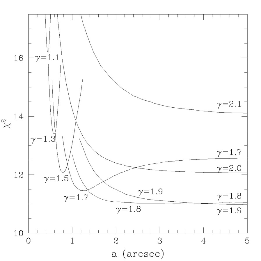 |
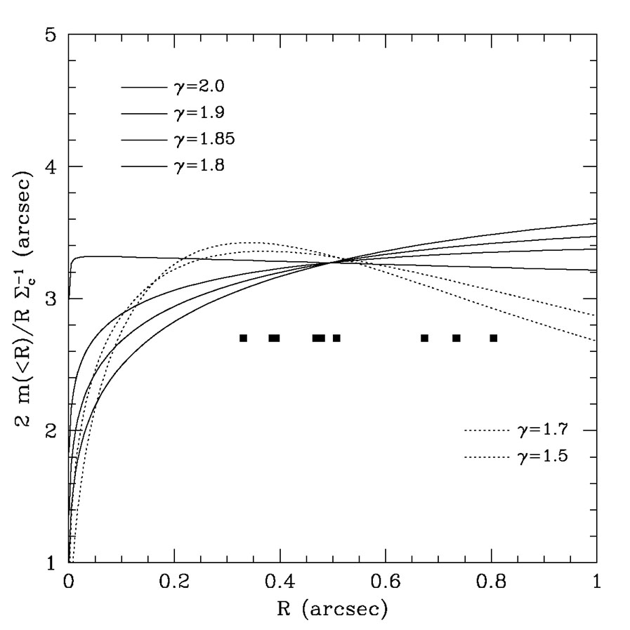
Figure B.24. (Top) Goodness of fit
|
The reason it is wrong and cannot be used to compute parameter errors is
that the uncertainty
i in the
image positions does not have any meaning
on the source plane. This is easily understood if we Taylor expand the
lens equation near the projected source point
i corresponding to an image
 |
(B.82) |
where Mi-1 is the inverse magnification
tensor at the observed location
of the image. In the frame where the tensor is diagonal, we have that

 ± =
± =
 ±
±
 ± so a
positional error
± on the source plane corresponds to a
positional error ±-1
± on the image plane. Since the
observed lensed images are almost always magnified (usually
+ = 1 +
± so a
positional error
± on the source plane corresponds to a
positional error ±-1
± on the image plane. Since the
observed lensed images are almost always magnified (usually
+ = 1 +
 +
+
 ~ 1 and
0.5 > |-
= 1 + -
| <
0.05) there is always one direction in which
small errors on the source plane are significantly magnified when projected
back onto the image plane. Hence, if you find solutions with
2src ~
Ndof where Ndof is the number of
degrees of freedom, you will have source plane uncertainties
~ 1 and
0.5 > |-
= 1 + -
| <
0.05) there is always one direction in which
small errors on the source plane are significantly magnified when projected
back onto the image plane. Hence, if you find solutions with
2src ~
Ndof where Ndof is the number of
degrees of freedom, you will have source plane uncertainties
 i.
However, the actual
errors on the image plane are µ = | M| larger, so the
2 on the image
plane is ~ µ2 Ndof and you in
fact have a terrible fit.
i.
However, the actual
errors on the image plane are µ = | M| larger, so the
2 on the image
plane is ~ µ2 Ndof and you in
fact have a terrible fit.
If you assume that in any interesting model you are close to having a good solution, then this Taylor expansion provides a means of using the easily computed source plane positions to still get a quantitatively accurate fitting statistic,
 |
(B.83) |
in which the magnification tensor Mi is used to
correct the error in the source position to an error in the image
position. This procedure will be approximately correct provided the
observed and model image positions are close enough for the Taylor
expansion to be valid. Finally, there is the exact statistic where for
the model source position
you numerically solve the lens equation to find the exact image positions
i() and then compute the goodness of fit
on the image plane
 |
(B.84) |
This will be exact even if the Taylor expansion of
2int
is breaking down,
and if you find all solutions to the lens equations you can verify that
the model predicts no additional visible images. Unfortunately, using
the exact
2img
is also a much slower numerical procedure.
As we discussed earlier, even though lens models provide the most
accurate mass normalizations in astronomy, they can constrain the mass
distribution only if the source is more complex than a single compact
component. Here we only show examples where there are multiple point-like
components, deferring discussions of models with extended source structure
to Section B.10. The most spectacular
example of a multi-component source is B1933+503 (Sykes et al.
[1998],
see Fig. B.7)
where a source consisting of a radio core and
two radio lobes has 10 lensed images because the core and one lobe are
quadruply imaged and the other lobe is doubly imaged. Since we have
many images spread over roughly a factor of two in radius, this lens should
constrain the radial mass distribution just as in our discussion for
Section B.4.3. Muñoz et al.
([2001],
also see Cohn et al.
[2001]
for softened power law models) fitted this system with cuspy models
(Eqn. 55 with
 = 2 and m = 4),
varying the inner density slope n =
(
= 2 and m = 4),
varying the inner density slope n =
(
 r-n) and the break radius a.
Fig. B.24 shows the resulting
2 as a function
of the parameters and Fig. B.25 illustrates the
range of the
acceptable monopole mass distributions - both are very similar to
Fig. B.21. The best fit is for
= 1.85
with an allowed range of
1.6 <
< 2.0 that completely excludes the shallow
= 1 cusps
of the Hernquist and NFW profiles and is marginally consistent with the
= 2 cusp
of the SIS model.
A second example, which illustrates how the distribution of mass
well outside the region with images has little effect on the models,
are the Winn et al. (2003) models of the three-image lens PMNJ1632-0033
shown in Fig. B.26. In these models the outer
slope
r-n) and the break radius a.
Fig. B.24 shows the resulting
2 as a function
of the parameters and Fig. B.25 illustrates the
range of the
acceptable monopole mass distributions - both are very similar to
Fig. B.21. The best fit is for
= 1.85
with an allowed range of
1.6 <
< 2.0 that completely excludes the shallow
= 1 cusps
of the Hernquist and NFW profiles and is marginally consistent with the
= 2 cusp
of the SIS model.
A second example, which illustrates how the distribution of mass
well outside the region with images has little effect on the models,
are the Winn et al. (2003) models of the three-image lens PMNJ1632-0033
shown in Fig. B.26. In these models the outer
slope  , with
r- asymptotically, of the density was
also explored but has little effect on the results. Unless the break
radius of the profile is interior to the B image, the mass profile
is required to be close to isothermal
1.89 <
< 1.93.
, with
r- asymptotically, of the density was
also explored but has little effect on the results. Unless the break
radius of the profile is interior to the B image, the mass profile
is required to be close to isothermal
1.89 <
< 1.93.
 |
Figure B.26. Allowed parameters for cuspy
models of PMNJ1632-0033 assuming that image
C is a true third image. Each panel shows the constraints on the inner
density cusp |
Unfortunately, systems like B1933+503 and PMNJ1632-0033 are a small minority of lens systems. For most lenses, obtaining information on the radial density profile requires some other information such as a dynamical measurement (Section B.4.9), a time delay measurement (Section B.5) or a lensed extended component of the source (Section B.10). Even for these systems, it is important to remember that the actual constraints on the density structure really only apply over the range of radii spanned by the lensed images - the mass interior to the images is constrained but its distribution is not, while the mass exterior to the images is completely unconstrained. This is not strictly true when we include the angular structure of the gravitational field and the mass distribution is quasi-ellipsoidal.
It is also important to keep some problems with parametric models in mind. First, models that lack the degrees of freedom needed to describe the actual mass distribution can be seriously in error. Second, models with too many degrees of freedom can be nonsense. We can illustrate these two limiting problems with the sad history of Q0957+561 for the first problem and attempts to explain anomalous flux ratios (see Section B.8) with complex angular structures in the density distribution for the dark matter for the second.
Q0957+561, the first lens discovered (Walsh, Carswell & Weymann [1979]) and the first lens with a well measured time delay (see Section B.5, Schild & Thomson [1970], Kundic et al. [1997] and references therein), is an ideal lens for demonstrating the trouble you can get into using parametric models without careful thought. The lens consists of a cluster and its brightest cluster galaxy with two lensed images of a radio source bracketing the galaxy. VLBI observations (e.g. Garrett et al. [1994]) resolve the two images into thin, multi-component jets with very accurately measured positions (uncertainties as small as 0.1 mas, corresponding to deflections produced by a mass scale ~ 10-8 of the primary lens!). Models developed along two lines. One line focused on models in which the cluster was represented as an external shear (e.g. Grogin & Narayan [1996], Chartas et al. [1998], Barkana et al. [1999], Chae [1999]) while the other explored more complex models for the cluster (see Kochanek [1991b], Bernstein, Tyson & Kochanek [1993], Bernstein & Fischer [1999]) and argued that external shear models had too few parameters to represent the mass distribution given the accuracy of the constraints. The latter view was born out by the morphology of the lensed host galaxy (Keeton et al. [2000]) and direct X-ray observations of the cluster (Chartas et al. [2002]) which showed that the lens galaxy was within about one Einstein radius of the cluster center where a tidal shear approximation fails catastrophically. The origin of the problem is that as a two-image lens, Q0957+561 is critically short of constraints unless the fine details of the VLBI jet structures are included in the models. Many studies imposed these constraints to the limit of the measurements while not including all possible terms in the potential which could produce a deflection on that scale (i.e. the precision should have been restricted to milli-arcseconds rather than micro-arcseconds). Models would adjust the positions and masses of the cluster and the lens galaxy in order to reproduce the small scale astrometric details of the VLBI jets without including less massive components of the mass distribution (e.g. the ellipticity gradient and isophote twist of the lens galaxy, Keeton et al. [2000]) that also affect the VLBI jet structure on these angular scales. Lens models must contain all reasonable structures producing deflections comparable to the scale of the measurement errors.
We are in the middle of an experiment exploring the second problem - if you include small scale structures but lack the constraints needed to measure them, their masses easily become unreasonable unless constrained by common sense, physical priors or additional data. Lately this has become an issue in studies (Evans & Witt [2003], Kochanek & Dalal [2004], Quadri, Moller & Natarajan [2003], Kawano et al. [2004]) of whether the flux ratio anomalies in gravitational lenses could be due to complex angular structure in the lens galaxy rather than CDM substructure or satellites in the lens galaxy (see Section B.8). The problem, as we discuss in the next section on non-parametric models (Section B.4.7), is that lens modeling with large numbers of parameters is closely related to solving linear equations with more variables than constraints - as the matrix inversion necessary to finding a solution becomes singular, the parameters of the mass distribution show wild, large amplitude fluctuations even as the fit to the constraints becomes perfect. Thus, a model including enough unconstrained parameters is guaranteed to "solve" the anomalous flux ratio problem even if it should not. For example, Evans & Witt ([2003]) could match the flux ratios of Q2237+0305 even though for this lens we know from the time variability of the flux ratios that the flux ratio anomalies are created by microlensing rather than complex angular structures in the lens model (see Part 4).
If only the four compact images are modeled, then the flux ratio
anomalies can be greatly reduced or eliminated in almost all lenses at the
price of introducing deviations from an ellipsoidal density distribution far
larger than expected (see Section B.4.4).
In some cases, however, you
can test these solutions because the lens has extra constraints beyond the
four compact images. We illustrate this in
Fig. B.27. By adding large amplitude
cos 3 and
cos 4 perturbations to
the surface density model for B1933+503, Kochanek & Dalal
([2004])
could reproduce the observed image flux ratios if they fit only the four
compact sources. However, after adding the constraints from the other
lensed components, the solution is driven back to being nearly
ellipsoidal and the flux ratios cannot be fit. In every case, Kochanek
& Dalal
([2004])
found that the extra constraints drove the solution back toward an
ellipsoidal
density distribution. In short, a sufficiently complex model can fit
underconstrained data, but that does not mean it makes any sense to do
so.
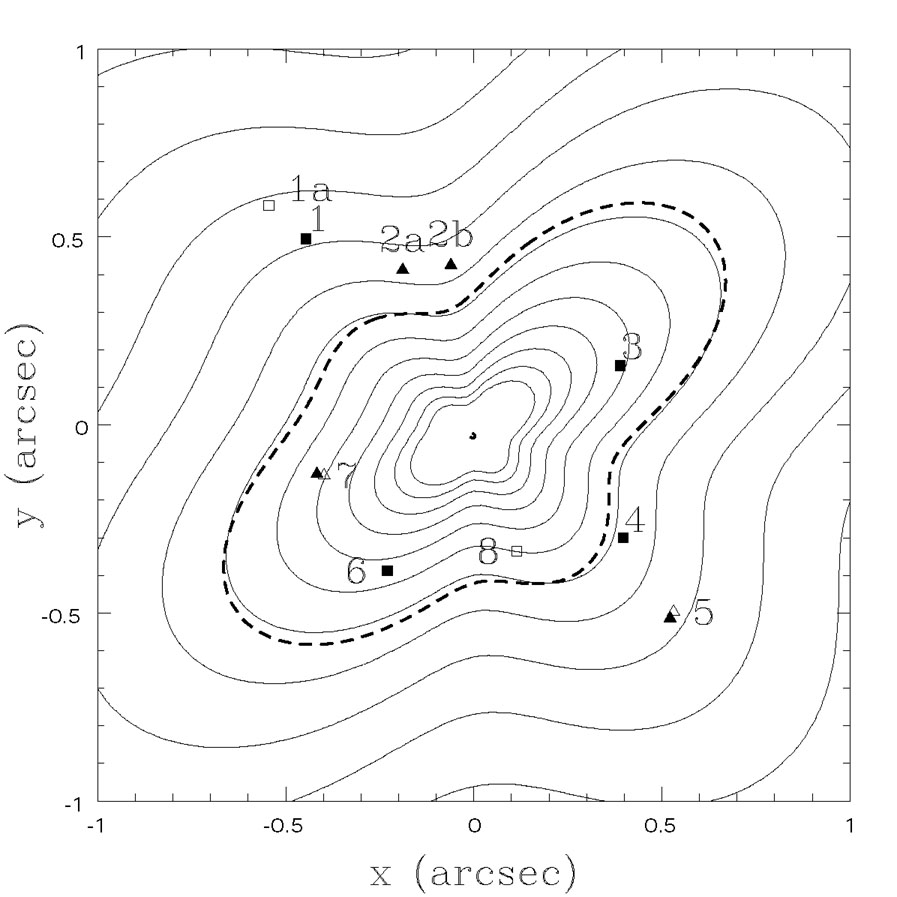 |
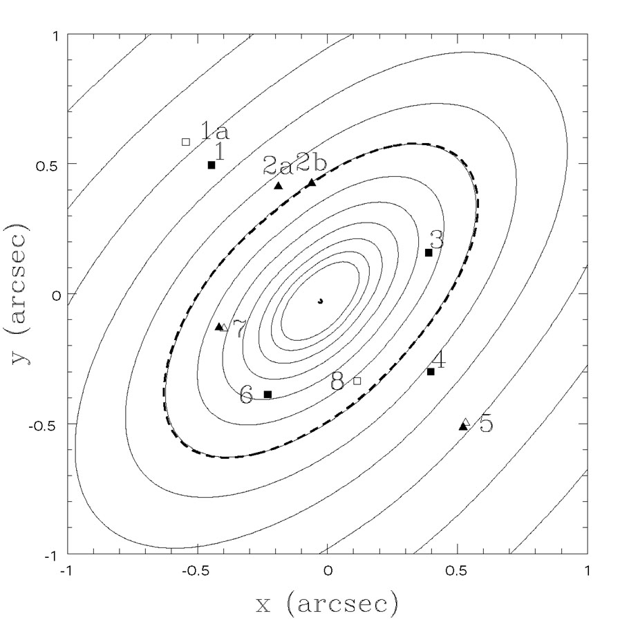 |
Figure B.27. Surface density contours for models of B1933+503 including misaligned a3 and a4 multipoles (thin lines). The model in the top panel is constrained only by the 4 compact images (images 1, 3, 4 and 6, filled squares). The model in the bottom panel is also constrained by the other images in the lens (the two-image system 1a/8, open squares; the four-image system 2a/2b/5/7 filled triangles; and the two-image system comprising parts of 5/7, open triangles) The tangential critical line of the model (heavy solid curve) must pass between the merging images 2a/2b, but fails to do so in the first model (top panel). |