


B.3.2. Circular Lenses
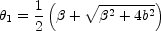
While one of the most important lessons about modeling gravitational
lenses in the real world is that you can never (EVER!)
2 safely neglect the
angular structure
of the gravitational potential, it is still worth starting with circular
lens models. They provide a basic introduction to many of the elements which
are essential to realistic models without the need for numerical
calculation. In a circular lens, the effective lens potential (Part 1)
is a function only of the distance from the lens center
 =
|
=
| |. Rays
are radially deflected by the angle
|. Rays
are radially deflected by the angle
 |
(B.3) |
where we recall from Part 1 that
 () =
() =
 () /
c is
the surface density in units of the critical surface density,
Dds and Ds
are the lens-source and observer-source comoving distances and
() /
c is
the surface density in units of the critical surface density,
Dds and Ds
are the lens-source and observer-source comoving distances and
 =
Ddang
is the proper distance from the lens.
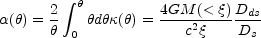
The bend angle is simply twice the Schwarzschild radius of the enclosed
mass,
4GM( < )
/ c2, divided by the impact
parameter and
scaled by the distance ratio Dds / Ds.
=
Ddang
is the proper distance from the lens.
The bend angle is simply twice the Schwarzschild radius of the enclosed
mass,
4GM( < )
/ c2, divided by the impact
parameter and
scaled by the distance ratio Dds / Ds.
The lens equation (see Part 1) becomes
 |
(B.4) |
where
 |
(B.5) |
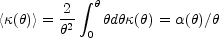
is the average surface density interior to
in units of the
critical density. Note that there must be a region with
<> > 1 to have
solutions on both sides
of the lens center. Because of the circular symmetry, all images
will lie on a line passing through the source and the lens center.
The inverse magnification tensor (or Hessian, see Part 1) also has a simple form, with
 |
(B.6) |
where =
(cos ,
sin). The
convergence (surface density) is
,
sin). The
convergence (surface density) is
 |
(B.7) |
and the shear is
 |
(B.8) |
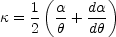
The eigenvectors of M-1 point in the radial and
tangential directions, with a radial eigenvalue of
 + =
1 - +
+ =
1 - +
 = 1 -
d
= 1 -
d /
d and a tangential
eigenvalue of
_ = 1 -
-
= 1 -
/
= 1 -
<>. If either one of
these eigenvalues is zero, the magnification diverges and we are on
either the radial or tangential critical curve. If we can resolve
the images, we will see the images radially magnified near the radial
critical curve and tangentially magnified near the tangential critical
curve. For example, all the quasar host galaxies seen in
Figs. B.3
and B.4
lie close to the tangential critical line and are stretched tangentially
to form partial or complete Einstein rings. The signs of the eigenvalues
± give
the parities of the images
and the type of time delay extremum associated with the images.
If both eigenvalues are positive, the image is a minimum. If both
are negative, the image is a maximum. If one is positive and the
other negative, the image is a saddle point. The inverse of the
total magnification
µ-1 = | M-1| is the product of
the eigenvectors,
so it is positive for minima and maxima and negative for saddle points.
The signs of the eigenvalues are referred to as the partial parities of
the images, while the sign of the total magnification is referred to as
the total parity.
/
d and a tangential
eigenvalue of
_ = 1 -
-
= 1 -
/
= 1 -
<>. If either one of
these eigenvalues is zero, the magnification diverges and we are on
either the radial or tangential critical curve. If we can resolve
the images, we will see the images radially magnified near the radial
critical curve and tangentially magnified near the tangential critical
curve. For example, all the quasar host galaxies seen in
Figs. B.3
and B.4
lie close to the tangential critical line and are stretched tangentially
to form partial or complete Einstein rings. The signs of the eigenvalues
± give
the parities of the images
and the type of time delay extremum associated with the images.
If both eigenvalues are positive, the image is a minimum. If both
are negative, the image is a maximum. If one is positive and the
other negative, the image is a saddle point. The inverse of the
total magnification
µ-1 = | M-1| is the product of
the eigenvectors,
so it is positive for minima and maxima and negative for saddle points.
The signs of the eigenvalues are referred to as the partial parities of
the images, while the sign of the total magnification is referred to as
the total parity.
It is useful to use simple examples to illustrate the behavior of circular
lenses for different density profiles. In most previous lensing reviews,
the examples are based on lenses with finite core radii. However, most
currently popular models of galaxies and clusters have central density cusps
rather than core radii, so we will depart from historical practice and
focus on the power-law lens (e.g. Evans & Wilkinson
[1998]).
Suppose, in three dimensions, that the lens has a density distribution

 r-n. Such a lens will produce deflections of
 |
(B.9) |
as shown in Fig. B.9, with convergence and shear profiles
 |
(B.10) |
The power law lenses cover most of the simple, physically interesting
models. The point mass lens is the limit
n  3, with
deflection
= b2
/ , convergence
= 0 (with a central
singularity) and shear
=
b2 / r2. The singular isothermal
sphere (SIS)
is the case with n = 2. It has a constant deflection
= b, and
equal convergence and shear
=
= b
/ 2. A uniform
critical sheet is the limit
n 1 with
=
,
= 1
and =
0. Models with n
3/2 have the cusp
exponent of the Moore
([1998])
halo model. The popular
1 / r NFW
(Navarro, Frenk & White
[1996],
see Section B.4.1) density cusps are not
quite the same as the
n 1 case
because the projected surface density of a
1 / r cusp has
ln rather
than a constant. Nonetheless, the behavior of the power law models as
n 1
will be very similar to the NFW model if the lens is dominated by the
central cusp. The central regions of galaxies probably act like cusps with
1
3, with
deflection
= b2
/ , convergence
= 0 (with a central
singularity) and shear
=
b2 / r2. The singular isothermal
sphere (SIS)
is the case with n = 2. It has a constant deflection
= b, and
equal convergence and shear
=
= b
/ 2. A uniform
critical sheet is the limit
n 1 with
=
,
= 1
and =
0. Models with n
3/2 have the cusp
exponent of the Moore
([1998])
halo model. The popular
1 / r NFW
(Navarro, Frenk & White
[1996],
see Section B.4.1) density cusps are not
quite the same as the
n 1 case
because the projected surface density of a
1 / r cusp has
ln rather
than a constant. Nonetheless, the behavior of the power law models as
n 1
will be very similar to the NFW model if the lens is dominated by the
central cusp. The central regions of galaxies probably act like cusps with
1  n
2.
n
2.
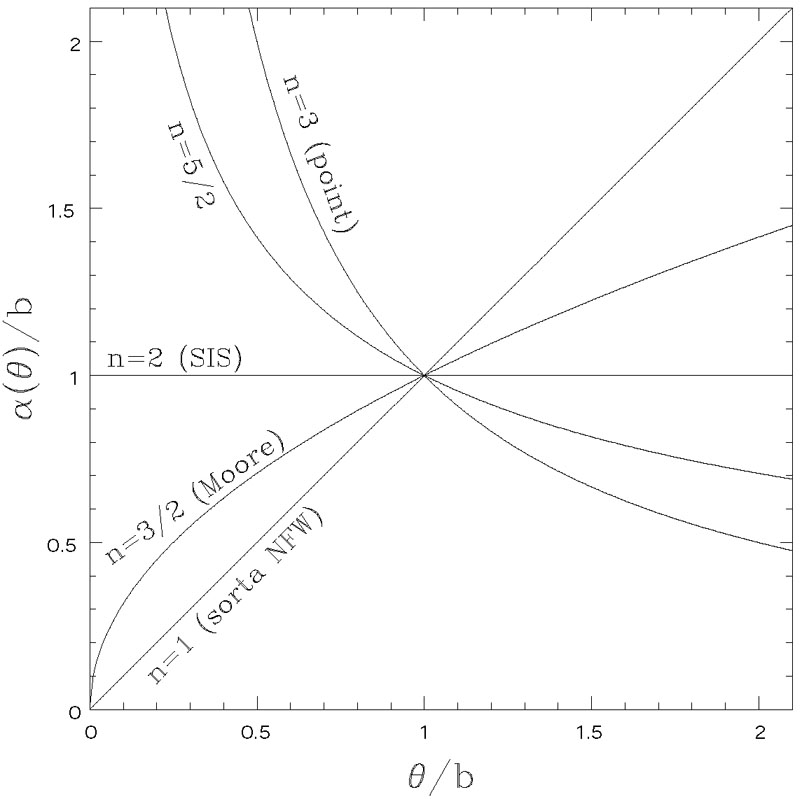 |
Figure B.9. The bending angles of the power law lens models. Profiles more centrally concentrated (n > 2) than the SIS (n = 2), have divergent central deflections, while profiles more extended (n < 2) than SIS have deflection profiles that become zero at the center of the lens. The n = 1 model is not quite an NFW model because the surface density is constant rather than logarithmic. |
The tangential magnification eigenvalue of these models is
 |
(B.11) |
which is always equal to zero at
= b
 E. This
circle defines the tangential critical curve or
Einstein (ring) radius of the lens. We normalized the models in this
fashion
because the Einstein radius is usually the best-determined parameter
of any lens model, in the sense that all successful models will find
nearly the same Einstein radius (e.g. Kochanek
[1991a],
Wambsganss & Paczynski
[1994]).
The source position corresponding
to the tangential critical curve is the origin
(
E. This
circle defines the tangential critical curve or
Einstein (ring) radius of the lens. We normalized the models in this
fashion
because the Einstein radius is usually the best-determined parameter
of any lens model, in the sense that all successful models will find
nearly the same Einstein radius (e.g. Kochanek
[1991a],
Wambsganss & Paczynski
[1994]).
The source position corresponding
to the tangential critical curve is the origin
( = 0), and the
reason the magnification diverges is that a point source at the
origin is converted into a ring on the tangential critical curve
leading to a divergent ratio between the "areas" of the source
and the image. The other important point to notice is that the mean
surface density inside the tangential critical radius is
<>
1
independent of the model. This is true of any
circular lens. With the addition of angular structure it is not
strictly true, but it is a very good approximation unless the mass
distribution is very flattened.
The definition of b in terms of the properties of the
lens galaxy will depend on the particular profile. For example, in a point
mass lens (n
3), b2 = (4GM / c2
Ddang)(Dds /
Ds) where M
is the mass, while in an SIS lens (n = 2),
b = 4
= 0), and the
reason the magnification diverges is that a point source at the
origin is converted into a ring on the tangential critical curve
leading to a divergent ratio between the "areas" of the source
and the image. The other important point to notice is that the mean
surface density inside the tangential critical radius is
<>
1
independent of the model. This is true of any
circular lens. With the addition of angular structure it is not
strictly true, but it is a very good approximation unless the mass
distribution is very flattened.
The definition of b in terms of the properties of the
lens galaxy will depend on the particular profile. For example, in a point
mass lens (n
3), b2 = (4GM / c2
Ddang)(Dds /
Ds) where M
is the mass, while in an SIS lens (n = 2),
b = 4 (
( v /
c)2
Dds / Ds where
v is the (1D)
velocity dispersion of the lens. For the other profiles, b
can be defined in terms of some velocity dispersion or mass estimate for
the lens, as we will discuss later in
Section B.4.9 and
Section B.6.
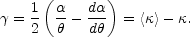
The radial magnification eigenvalue of these models is
v /
c)2
Dds / Ds where
v is the (1D)
velocity dispersion of the lens. For the other profiles, b
can be defined in terms of some velocity dispersion or mass estimate for
the lens, as we will discuss later in
Section B.4.9 and
Section B.6.
The radial magnification eigenvalue of these models is
 |
(B.12) |
which can be zero only if n < 2. If n < 2 the
deflection goes to zero at the origin and the lens has a
radial critical curve at
= b(2 -
n)1/(n-1) < b interior
to the tangential critical curve. Models with n
 2 have constant
(n = 2) or rising deflection profiles as we approach the lens center
and have negative derivatives
d /
d at all radii.
2 have constant
(n = 2) or rising deflection profiles as we approach the lens center
and have negative derivatives
d /
d at all radii.
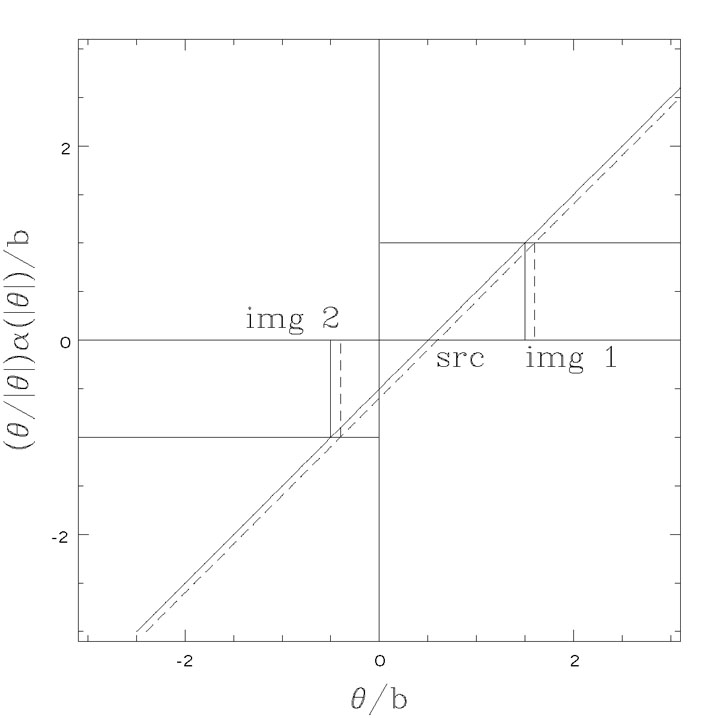
A nice property of circular lenses is that they allow simple graphical
solutions
of the lens equation for arbitrary deflection profiles. There are two parts
to the graphical solution - the first is to determine the radial positions
i of the
images given a source position
, and the
second is to determine the magnification by comparing the area of the
images to the area of the source. Recall first, that by symmetry, all
the images must lie on a line passing through the source and the lens. Let
now be
a signed radius that is positive along this line on one side of the lens
and negative on the other. The lens equation (Eqn.B.4) along the line is
simply
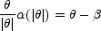 |
(B.13) |
where we have rearranged the terms to put the deflection on one side and the
image and source positions on the other. One side of the equation is
the bend angle (Fig. B.9), while the other side
of the equation, -
, is simply a
line of unit slope passing through the source position
. The
solutions to the lens equation for any source position
are the
radii i where
the line crosses the curve.
For understanding any observed lens, it is always useful to first sketch
where
the critical lines must lie. Recall from the discussion of caustics in
Part 1, that images are always created and destroyed on critical lines
as the source crosses a caustic, so the critical lines and caustics define
the general structure of the lens. All our power law models have a
tangential critical line at
= b, which is
the solution
(b) = b
and corresponds to the source position
= 0. The
origin, as the
projection of the critical curve onto the source plane, is the tangential
caustic (strictly speaking a degenerate pseudo-caustic) corresponding to
the critical line. A point source at the
origin is transformed into an Einstein ring of radius
E = b.
The second step of the graphical construction is to determine the angular
structure of the image. For simplicity, suppose the source is an arc with
radial width  and angular
width
. By symmetry,
the angle subtended by an image relative to the lens center must be
the same as that subtended by the source. For an image at
i and a source at
, the
tangential extent of the image is
|i|
while that of
the source is
.
The tangential magnification of the image is simply
|i| /
= (1 -
|(i) /
i|)-1 after making
use of the lens equation (Eqn. B.13), and this is identical to the
tangential magnification eigenvalue (Eqn. B.11). The thickness of
the arc requires finding the image radii for the inner and outer edges
of the source,
i() and
i( +
). The ratio
of the thickness of the two arcs is the radial magnification,
and angular
width
. By symmetry,
the angle subtended by an image relative to the lens center must be
the same as that subtended by the source. For an image at
i and a source at
, the
tangential extent of the image is
|i|
while that of
the source is
.
The tangential magnification of the image is simply
|i| /
= (1 -
|(i) /
i|)-1 after making
use of the lens equation (Eqn. B.13), and this is identical to the
tangential magnification eigenvalue (Eqn. B.11). The thickness of
the arc requires finding the image radii for the inner and outer edges
of the source,
i() and
i( +
). The ratio
of the thickness of the two arcs is the radial magnification,
 |
(B.14) |
and this is simply the inverse of the radial eigenvalue of the
magnification matrix (Eqn. B.12) where we have taken the derivative of
the lens equation (Eqn. B.13) with respect to
the source position to obtain the final result. Thus, the tangential
magnification simply reflects the fact that the angle subtended by the
source is the angle subtended by the image, while the radial magnification
depends on the slope of the deflection profile with declining
deflection profiles
(d /
d < 0)
demagnifying the source and rising profiles magnifying the source.
 |
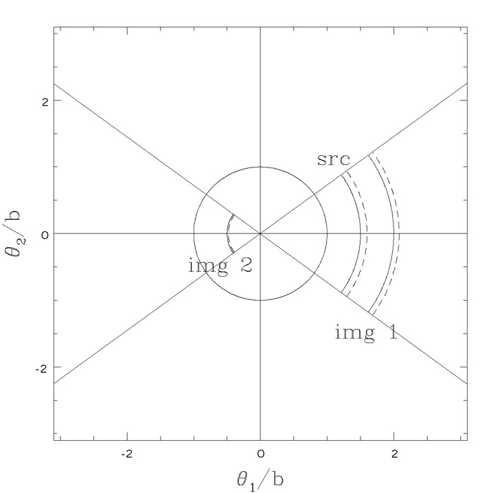 |
Figure B.10. Graphical solutions for the point mass (n = 3) lens. The top panel shows the graphical solution for the radial positions of the images, and the bottom panel shows the graphical solution for the image structure. Note the strong radial demagnification of image 2 produced by the falling deflection profile. |
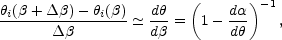
In Fig. B.10 we illustrate this for the point
mass lens (n 3).
From the shape of the deflection profile, it is immediately obvious
that there will be only two images, one on each side of the lens. If
we assume
> 0, the first image is a minimum located at
 |
(B.15) |
with 1 >
E and
positive magnification
 |
(B.16) |
while the second image is a saddle point located at
 |
(B.17) |
with - E <
2 < 0 and
negative magnification
 |
(B.18) |
As the source approaches the tangential caustic
(
0) the
magnifications of both images diverge as
-1
and the image radii
converge to E.
As the source moves to infinity, the magnification
of the first image approaches unity and its position approaches that of the
source, while the second image is demagnified by the factor (1/2)(b
/ )
and converges to the position of the lens. The image separation
 |
(B.19) |
is always larger than the diameter of the Einstein ring and the total magnification
 |
(B.20) |
is the characteristic light curve expected for isolated Galactic microlensing events (see Part 4). The point mass lens has one peculiarity that makes it different from extended density distributions like galaxies in that it has two images independent of the impact parameter of the source and no radial caustic. This is a characteristic of any density distribution with a divergent central deflection (n > 2).
 |
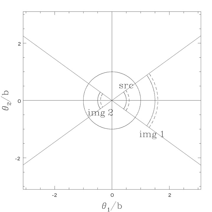 |
Figure B.11. Graphical solutions for the SIS
(n = 2) lens when
|
 |
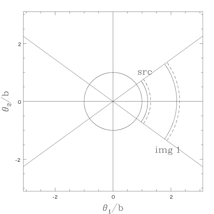 |
Figure B.12. Graphical solutions for the SIS
(n = 2) lens when
|
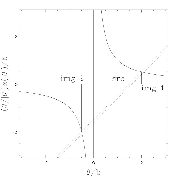
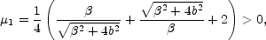
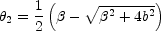
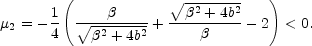
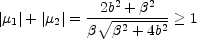
The SIS (n = 2) model is the "standard" lens model for galaxies.
Figs. B.11 and B.12
show the geometric constructions for the images of an SIS lens.
If 0 < <
b, then the SIS lens also produces two images
(Fig. B.11). The first image is a minimum
located at
 |
(B.21) |
and the second image is a saddle point located at
 |
(B.22) |
The image separation
|1 -
2| =
2b is constant, and the total magnification
|µ1| + |µ2| = 2b /
is a simple
power law. The magnification produced by an SIS lens is purely tangential
since the radial magnification is unity. If, however,
> b,
then there is only one image, corresponding to the minimum located
on the same side of the lens as the source (see
Fig. B.12). This boundary on the source plane at
= b
between having two images
at smaller radii and only one image at larger radii is a
radial (pseudo)-caustic that can be thought of as being associated
with a radial critical curve at the origin. It is a pseudo-caustic
because there are neither images nor a divergent magnification associated
with it.
 |
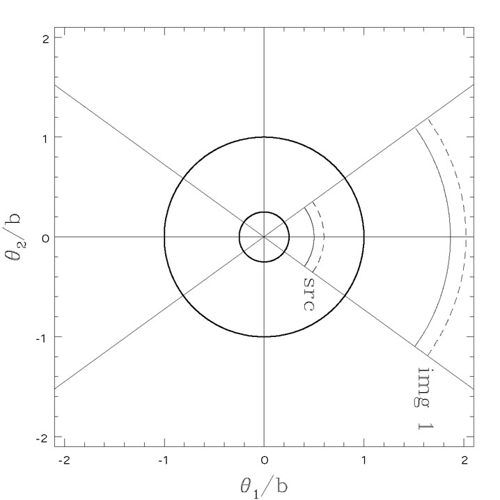 |
Figure 13. Graphical solutions for the
Moore profile cusp (n = 3/2) lens
when |
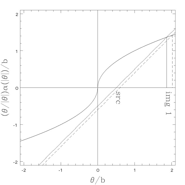
Historically the next step is to introduce a core radius to have a model
with a true radial critical line and caustic (see Part 1, Blandford
& Kochanek
[1987b],
Kochanek & Blandford
[1987],
Kovner
[1987a],
Hinshaw & Krauss
[1987],
Krauss & White
[1992],
Wallington & Narayan
[1993],
Kochanek
[1996a]).
Instead we will consider the still softer power law model with n
= 3/2, which would correspond to the central exponent of the "Moore"
profile proposed for CDM halos (Moore et al.
[1998]).
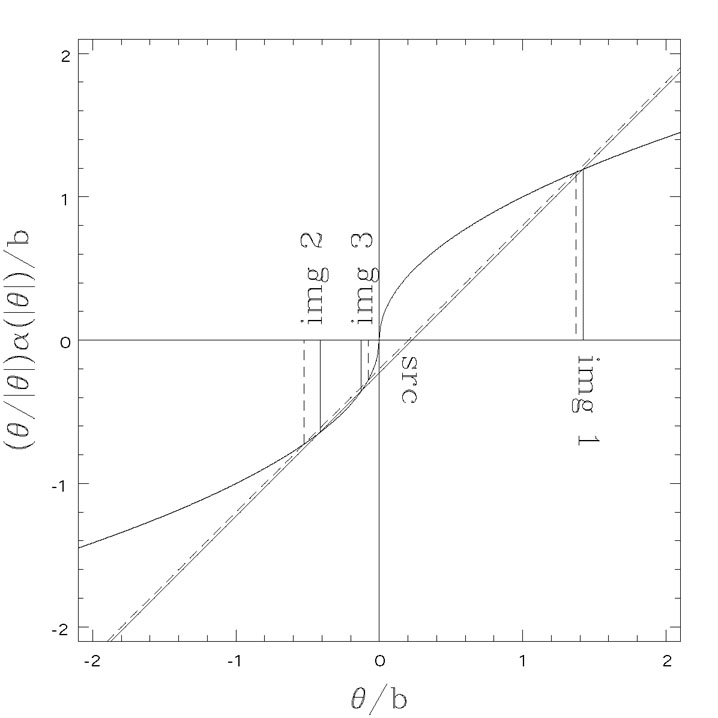
As fig. B.13 shows, there is only one solution
for || >
b / 4, a minimum located at
 |
(B.23) |
and with 1 >
b assuming
is positive.
The magnification expressions are too complex to be of much use,
but the magnification µ1 diverges at
= b when the
source is on the tangential pseudo-caustic at
= 0. As
Fig. B.14 shows, we
find two additional images once
|| <
b / 4. The first additional image is a saddle point located at
 |
(B.24) |
with - b <
2 < -
b / 4,
which has a negative magnification that diverges at both
2 = -
b (the tangential critical curve) and
2 = -
b / 4. This latter radius defines the
radial critical curve where the magnification diverges because the
radial magnification eigenvalue
1 - +
= 1 -
d /
d = 0 at radius
= b / 4.
The third image is a maximum located at
 |
(B.25) |
with - b / 4 <
2 < 0 and
a positive magnification that diverges on the radial critical curve.
As we move the source outward from the center we would see images 2 and 3
approach each other, merging on the radial critical line where they would
have divergent magnifications, and then vanishing to leave only image 1.
We would see the same pattern if instead of softening the exponent we had
followed the traditional path and added a core radius to the SIS model.
With a finite core radius the central deflection profile would pass through
zero, and this would introduce a radial critical curve and a third image
which would be a maximum of the time delay surface.
 |
 |
Figure B.14. Graphical solutions for the
Moore profile cusp (n = 3/2) lens
when |
In Fig. B.14 we also illustrate the geometric meaning of the partial parities (the signs of the magnification eigenvalues). A source structure (the L) defines the reference shape. Image 1 is a minimum with positive partial parities (+ +) defined by the signs of the tangential and radial eigenvalues. The orientation of image 1 is the same as the source. Image 2 is a saddle point with mixed partial parities (- +) because the tangential eigenvalue is negative while the radial eigenvalue is positive. This means that the image is inverted in the tangential direction relative to the source. Image 3 is a maximum with negative partial parties (- -), so the image is inverted in both the radial and tangential directions relative to the source. The total parity, the product of the partial parities, is positive for maxima and minima so the orientation of the image can be produced by rotating the source. The total parity of the saddle point image is negative, so its orientation cannot be produced by a rotation of the source.
2 AND I MEAN EVER! DON'T EVEN THINK OF IT! Back.