B.3.3. Non-Circular Lenses

The tangential pseudo-caustic at the origin producing Einstein ring images is unstable to the introduction of any angular structure into the gravitational potential of the lens. There are two generic sources of angular perturbations. The first source of angular perturbations is the ellipticity of the lens galaxy. What counts here is the ellipticity of the gravitational potential rather than of the surface density. For a lens with axis ratio q, ellipticity = 1 - q, or eccentricity e = (1 - q²)^1/2, the ellipticity of the potential is usually ~ / 3 - potentials are always rounder than densities. The second source of angular perturbations is tidal perturbations from any nearby objects. This is frequently called the "external shear" or the "tidal shear" because it can be modeled as a linear shearing of the deflections. In all known lenses, quadrupole perturbations (i.e. cos(2) where is the azimuthal angle) dominate - higher order multipoles are certainly present and they can be quantitatively important, but they are smaller. For example, in an ellipsoid the amplitude of the cos 2m multipole scales as ^m (see Section B.4.4 and Section B.8).

Unfortunately, there is no example of a non-circular lens that can be solved in full generality unless you view the nominally analytic solutions to quartic equations as helpful. We can make the greatest progress for the case of an SIS in an external (tidal) shear field. Tidal shear is due to perturbations from nearby objects and its amplitude can be determined by Taylor expanding its potential near the lens (see Part 1 and Section B.4). Consider a lens with Einstein radius _E perturbed by an object with effective lens potential a distance _p away. For _E << _p we can Taylor expand the potential of the nearby object about the center of the primary lens, dropping the leading two terms. ³ This leaves, as the first term with observable consequences,

(B.26)

where _p is the surface density of the perturber at the center of the lens galaxy and _p > 0 is the tidal shear from the perturber. If the perturber is an SIS with critical radius b_p and distance _p from the primary lens, then _p = _p = b_p / 2_p. With this normalization, the angle _p points toward the perturber. For a circular lens, the shear _p = <> - can be expressed in terms of the surface density of the perturber, and it is larger (smaller) than the convergence if the density profile is steeper (shallower) than isothermal.

The effects of _p are observable only if we measure a time delay or have an independent estimate of the mass of the lens galaxy, while the effects of the shear are easily detected from the relative positions of the lensed images (see Part 1). Consider, for example, one component of the lens equation including an extra convergence,

(B.27)

and then simply divide by 1 - _p to get

(B.28)

The rescaling of the source position ₁ / (1 - _p) has no consequences since the source position is not an observable quantity, while the rescaling of the deflection is simply a change in the mass of the lens. This is known as the "mass sheet degeneracy" because it corresponds to adding a constant surface density sheet to the lens model (Falco, Gorenstein & Shapiro [1985], see Part 1), and it is an important systematic problem for both strong lenses and cluster lenses (see Part 3).

Thus, while the extra convergence can be important for the quantitative understanding of time delays or lens galaxy masses, it is only the shear that introduces qualitatively new behavior to the lens equations. The effective potential of an SIS lens in an external shear is = b + ( / 2) ² cos 2 leading to the lens equations

(B.29)

where for > 0 the perturber is due North (or South) of the lens. The inverse magnification is

(B.30)

where = (₁, ₂) = (cos, sin).

The first step in any general analysis of a new lens potential is to locate the critical lines and caustics. In this case we can easily solve µ^-1 = 0 to find that the tangential critical line

(B.31)

is an ellipse whose axis ratio is determined by the amplitude of the shear and whose major axis points toward the perturber. We call it the tangential critical line because the associated magnifications are nearly tangential to the direction to the lens galaxy and because it is a perturbation to the Einstein ring of a circular lens. The tangential caustic, the image of the critical line on the source plane, is a curve called an astroid (Fig. B.15, it is not a "diamond" despite repeated use of the term in the literature). The parametric expression for the astroid curve is

(B.32)

where the parameter is the same as the angle appearing in the critical curve (Eqn. B.31) and we have defined _± = 2b / (1 ± ) for the locations of the cusp tips on the axes. The astroid consists of 4 cusp caustics on the symmetry axes of the lens connected by fold caustics with a major axis pointing toward the perturber. Like the SIS model without any shear, the origin plays the role of the radial critical line and there is a circular radial pseudo-caustic at = b.

As mentioned earlier, there is no useful general solution for the image positions and magnifications. We can, however, solve the equations for a source on one of the symmetry axes of the lens. For example, consider a solution on the minor axis of the lens (₂ = 0 for > 0). There are two ways of solving the lens equation to satisfy the criterion. One is to put the images on the same axis (₂ = 0) and the other is to place them on the arc defined by 0 = 1 + - b / . The images with ₂ = 0 are simply the SIS solutions corrected for the effects of the shear. Image 1 is defined by

(B.33)

and image 2 is defined by

(B.34)

Image 1 exists if ₁ > - b, it is a saddle point for - b < ₁ < - ₊ and it is a minimum for ₁ > - ₊. Image 2 has the reverse ordering. It exists for ₁ < b, it is a saddle point for ₊ < ₁ < b and it is a minimum for ₁ < ₊. The magnifications of both images diverge when they are on the tangential critical line (₁ = - ₊ for image 1 and ₁ = + ₊ for image 2) and approach zero as they move into the core of the lens (₁ - b for image 1 and ₁ + b for image 2). These two images shift roles as the source moves through the origin. The other two solutions are both saddle points, and they exist only if the source lies inside the astroid (|₁| < ₊ along the axis). The positions of images 3 (+) and 4 (-) are

(B.35)

and they have equal magnifications

(B.36)

The magnifications of the images diverge when the source reaches the cusp tip (|₁| = ₊) and the image lies on the tangential critical curve.

Thus, if we start with a source at the origin we can follow the changes in the image structure (see Fig. B.15, B.16). With the source at the origin we see 4 images on the symmetry axes with reasonably high magnifications, | µ_i| = (2 / ) / (1 - ²) ~ 10. It is a generic result that the least magnified four-image system is found for an on-axis source, and this configuration has a total magnification of order the inverse of the ellipticity of the gravitational potential. As we move the source toward the tip of the cusp ( ₊, Fig. B.15), image 1 simply moves out along the symmetry axis with slowly dropping magnification, while images 2, 3 and 4 move toward a merger on the tangential critical curve at = (- ₊, 0). Their magnifications steadily rise and then diverge when the source reaches the cusp. If we move the source further outward we find only images 1 and 2 with 1 moving outward and 2 moving inward toward the origin. As it approaches the origin, image 2 becomes demagnified and vanishes when b. Had we done the same calculation on the major axis (Fig. B.16), there is a qualitative difference. As we moved image 1 outward along the ₂ axis, image 3 and 4 would merge with image 1 when the source reaches the tip of the cusp at ₂ = _ rather than with image 2.

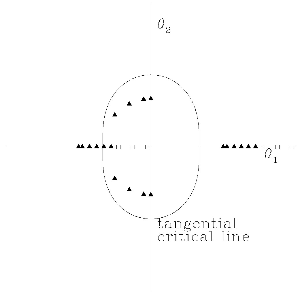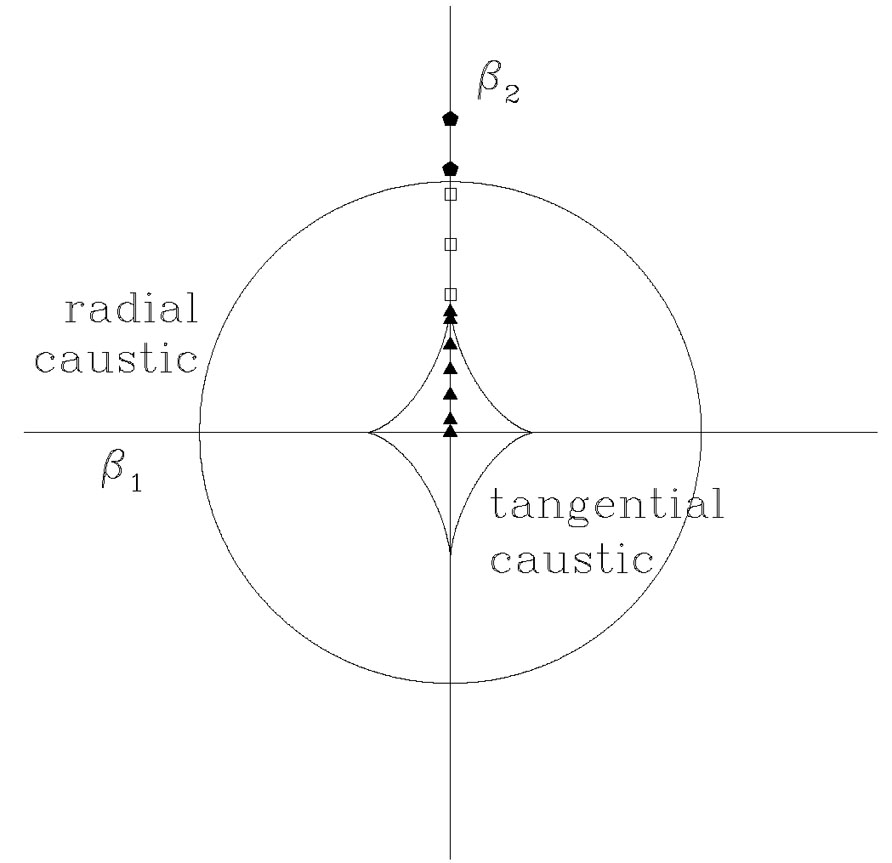
Figure B.15. Example of a minor axis cusp on the source (top) and image (bottom) planes. When the source is inside both the radial and tangential caustics (triangles) there are four images. As the source moves toward the cusp, three of the images head towards a merger on the critical line and become highly magnified to leave only one image once the source crosses the cusp and lies between the two caustics (open squares). In a minor axis cusp, the image surviving the cusp merger is a saddle point interior to the critical line. As the source approaches the radial caustic, one image approaches the center of the lens and then vanishes as the it crosses the caustic to leave only one image (pentagons).

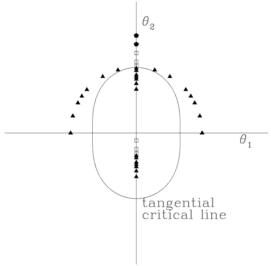Figure B.16. Example of a major axis cusp on the source (top) and image (bottom) planes. When the source is inside both the radial and tangential caustics (triangles) there are four images. As the source moves toward the cusp, three of the images head towards a merger on the critical line and become highly magnified to leave only one image once the source crosses the cusp and lies between the two caustics (open squares). In a major axis cusp, the image surviving the cusp merger is the minimum corresponding to the image we would see in the absence of a lens. As the source approaches the radial caustic, one image approaches the center of the lens and then vanishes as the source crosses the caustic to leave only one image (pentagons).

Unfortunately once we move the source off a symmetry axis, there is no simple solution. It is possible to find the locations of the remaining images given that two images have merged on the critical line, and this is useful for determining the mean magnifications of the lensed images, a point we will return to when we discuss lens statistics in Section B.6. Here we simply illustrate (Fig. B.17) the behavior of the images when we move the source radially outward from the origin away from the symmetry axes. Rather than three images merging on the tangential critical line as the source approaches the tip of a cusp, we see two images merging as the source approaches the fold caustic of the astroid. This difference, two images merging versus three images merging, is a generic difference between folds and cusps as discussed in Part 1. All images in these four-image configurations are restricted to an annulus of width ~ b around the critical line, so the mean magnification of all four image configurations is also of order ^-1 (see Finch et al. [2002]).

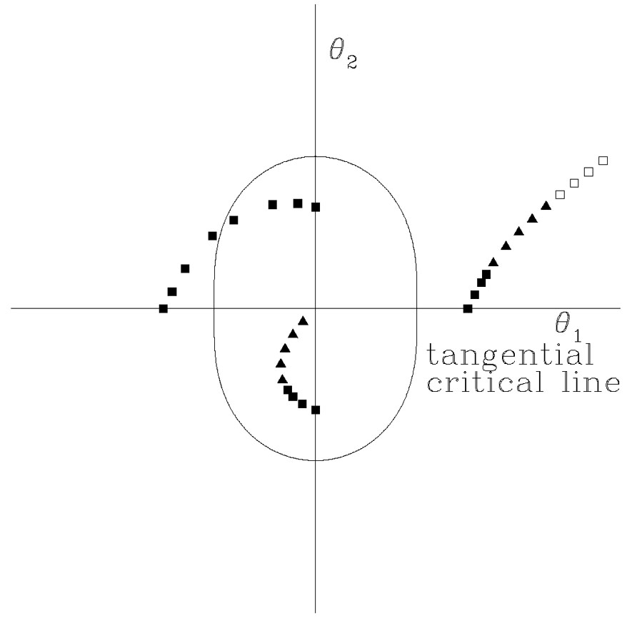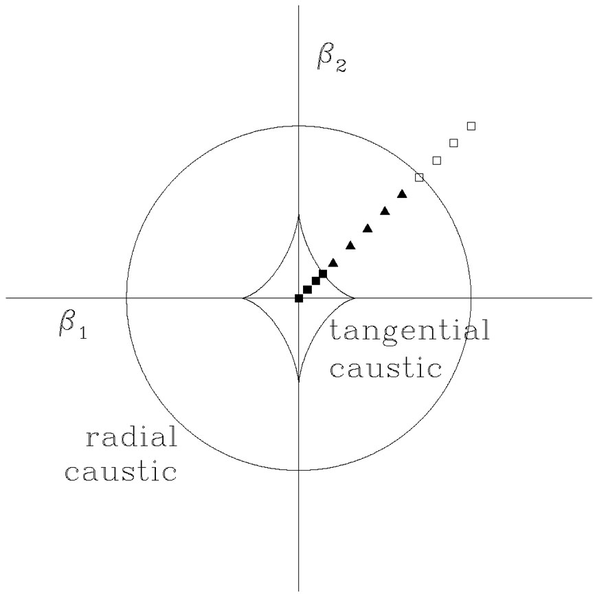
Figure B.17. Example of a fold merger on the source (top) and image (bottom) planes. When the source is inside both the radial and tangential caustics (filled squares) there are four images. As the source crosses the tangential caustic, two images merge, become highly magnified and then vanish, leaving only two images (triangles) when the source is outside the tangential caustic but inside the radial caustic. As the source approaches the radial caustic, one image moves into the center of the lens and then vanishes when the source crosses the radial caustic to leave only one image when the source is outside both caustics (open squares).

There is one more possibility for the caustic structure of the lens if the external shear is large enough. For 1/3 < || < 1, the tip of the astroid caustic extends outside the radial caustic, as shown if Fig. B.18. This allows a new image geometry, known as the cusp or disk geometry, where we see three images straddling the major axis of a very flattened potential. It is associated with the caustic region inside the astroid caustic but outside the radial caustic. This configuration appears to be rare for lenses produced by galaxies, with APM08279+5255 as the only likely candidate, but relatively more common in clusters. The difference is that clusters tend to have shallower density profiles than galaxies, which shrinks the radial caustics relative to the tangential caustics to allow more cross section for this image configuration and lower ellipticity thresholds before it becomes possible (Oguri & Keeton [2004] most recently, but also see Kochanek & Blandford [1987], Kovner [1987a], Wallington & Narayan [1993]).

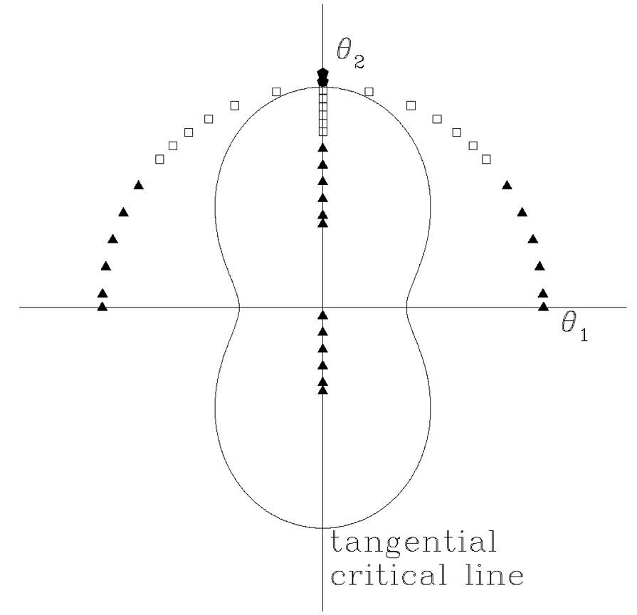Figure B.18. Example of a cusp or disk image geometry on the source (top) and image (bottom) planes. The shear is high enough to make the tangential caustic extend outside the radial caustic. For a source inside both caustics (triangles) we see a standard four-image geometry as in Fig. B.16. However, for a source outside the radial caustic but inside the tangential caustic (squares) we have three images all on one side of the lens. This is known as the cusp geometry because it is always associated with cusps, and the disk geometry because flattened disks are the only natural way to produce them. Once the source is outside the cusp tip (pentagon), a single image remains.

In general, it is far more difficult to analyze ellipsoidal lenses, in part because few ellipsoidal lenses have analytic expressions for their deflections. The exception is the isothermal ellipsoid (Kassiola & Kovner [1993], Kormann, Schneider & Bartelmann [1994], Keeton & Kochanek [1998]), including a core radius s, which is both analytically tractable and generally viewed as the most likely average mass distribution for gravitational lenses. The surface density of the isothermal ellipsoid

(B.37)

depends on the axis ratio q and the core radius s. For q = 1 - < 1 the major axis is the ₁ axis and s is the major axis core radius. The deflections produced by this lens are remarkably simple,

(B.38)

The effective lens potential is cumbersome but analytic,

(B.39)

the magnification is simple

(B.40)

and becomes even simpler in the limit of a singular isothermal ellipsoid (SIE) with s = 0 where µ^-1 1 - b / . In this case, contours of surface density are also contours of the magnification, and the tangential critical line is the = 1/2 isodensity contour just as for the SIS model. The critical radius scale b can be related to the circular velocity in the plane of the galaxy relatively easily. For an isothermal sphere we have that b_SIS = 4(_v / c)² D_ds / D_s where the circular velocity is v_c = 2^1/2 _v. For the projection of a three-dimensional (3D) oblate ellipsoid of axis ratio q₃ and inclination i, so that q² = q₃² cos²i + sin² i, the deflection scale is b = b_SIS(e₃ / sin^-1 e₃) where e₃ = (1 - q₃²)^1/2 is the eccentricity of 3D mass distribution. In the limit that q₃ 0 the model becomes a Mestel ([1963]) disk, the infinitely thin disk producing a flat rotation curve, and b = 2b_SIS / (see Section B.4.9 and Keeton, Kochanek & Seljak [1997], Keeton & Kochanek [1998], Chae [2003]). At least for the case of a face-on disk, at fixed circular velocity you get a smaller Einstein radius as you make the 3D distribution flatter because a thin disk requires less mass to produce the same circular velocity.

We can generate several other useful models from the isothermal ellipsoids. For example, steeper ellipsoidal density distributions can be derived by differentiating with respect to s². The most useful of these is the first derivative with ^-3/2 which is related to the Kuzmin ([1956]) disk (see Kassiola & Kovner [1993], Keeton & Kochanek [1998]). It is also easy to generate models with flat inner rotation curves and truncated halos by taking the difference of two isothermal ellipsoids. In particular if (s) is an isothermal ellipsoid with core radius s, the model

(B.41)

with a > s has a central core region with a rising rotation curve for s, a flat rotation curve for s a and a dropping rotation curve for a. In the singular limit (s 0), it becomes the "pseudo-Jaffe model" corresponding to a 3D density distribution (r² + s²)^-1(r² + a²)^-1 whose name derives from the fact that it is very similar the Jaffe model with r^-2(r + a)^-2 (Kneib et al. [1996], Keeton & Kochanek [1998]). We will discuss other common lens models in Section B.4.1.

The last simple analytic models we mention are the generalized singular isothermal potentials of the form = F() with surface density (, ) = (1/2)(F() + F''()) / . Both the SIS and SIE are examples of this model. The generalized isothermal sphere has a number of useful analytic properties. For example, the magnification contours are isodensity contours

(B.42)

with the tangential critical line being the contour with = 1/2, and the time delays between images depend only on the distances from the images to the lens center (see Witt, Mao & Keeton [2000], Kochanek, Keeton & McLeod [2001], Wucknitz [2002], Evans & Witt [2003]).

³ The first term, a constant, gives an equal contribution to the time delays of all the images, so it is unobservable when all we can measure is relative delays. The second term is a constant deflection, which is unobservable when all we can measure is relative deflections. Back.