8. THE ROLE OF SUBSTRUCTURE

Simulations of CDM halos predicted many more small satellites than were actually observed in the Milky Way (e.g. Kauffmann et al. [1993], Moore et al. [1999], Klypin et al. [1999]). Crudely 5-10% of the mass was left in satellites with perhaps 1-2% at the projected separations of 1-2R_e where we see most lensed images (e.g. Zentner & Bullock [2003], Mao et al. [2004]). This is far larger than the observed fraction of 0.01-0.1% in observed satellites (e.g. Chiba [2002]). Solutions were proposed in three broad classes: hide the satellites by preventing star formation so they are present but dark (e.g. Klypin et al. [1999], Bullock et al. [2000]), destroy them using self-interacting dark matter (e.g. Spergel & Steinhardt [2000]), or avoid forming them by changing the power spectrum to something similar to warm dark matter with significantly less power on the relevant mass scales (e.g. Bode et al. [2001]). These hypotheses left the major observational challenge of distinguishing dark satellites from non-existent ones. This became known as the CDM substructure problem.

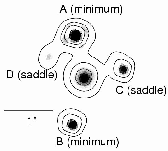Figure B.58. The most spectacular example of an anomalous flux ratio, SDSS0924+0219 (Inada et al. 2003). In this CASTLES infrared HST image, the D image should be comparable in brightness to the A image, but is actually an order of magnitude dimmer. The A and B images are minima, while C and D are saddle points. The contours are spaced by factors of two from the peak of the A image. The lens galaxy is seen at the center. At present we do not know whether the suppression of the saddle point in this lens is due to microlensing or substructure. If it is microlensing, ongoing monitoring programs should see it return to its expected flux within approximately 10 years.

It was well known in the lensing community that the fluxes of lensed images were usually poorly fit by lens models. There was a long litany of reasons for ignoring them arising from possible systematic errors which can corrupt image fluxes. Differential effects between the images from the interstellar medium of the lens can corrupt the fluxes (dust in the optical/IR, scatter broadening in the radio, see Section B.9.1). Time delays combined with source variability can corrupt any single-epoch measurement. Microlensing by the stars in the lens galaxy can modify the fluxes of any sufficiently compact component of the source (at a minimum the quasar accretion disk, see Part 4). The most peculiar problem was the of anomalous flux ratios in radio lenses. Radio sources are essentially unaffected by the ISM of the lens galaxy in low resolution observations that minimize the effects of scatter broadening (VLA rather than VLBI), true absorption appears to be rare, radio sources generally show little variability even when monitored, and most of the flux should come from regions too large to be affected by microlensing. Yet in B1422+231, for example, the three cusp images violated the cusp relation for their fluxes (that the sum of the signed magnifications of the three images should be zero, see Metcalf & Zhao [2002], Keeton, Gaudi & Petters [2003], or Schneider, Ehlers & Falco [1992]). ⁸

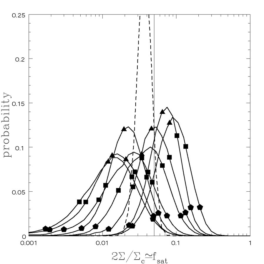
Figure B.59. (Top) A Monte Carlo test for estimating substructure surface densities. The heavy curves show the estimated probability distribution for the substructure surface density fraction in a sample of 7 four-image lenses in which the input fraction was 5% (marked by the vertical line). The points on the curve show the median, 1 and 2 confidence limits. The output distributions are consistent with the true input fraction. The dashed line shows how the accuracy would improve given a sample of 56 lenses (i.e. multiplying the 8 trials of 7 images each). Figure B.60. (Bottom) The same method applied to the real data. The three distributions show the effects of changing assumptions on the actual flux measurement errors - the greater the measurement uncertainties the less substructure surface density is required to explain the flux ratio anomalies. The middle case (10%) is probably slightly too conservative (20% is ridiculously conservative and 5% is probably too optimistic).

It is easier to outline the problem of anomalous flux ratios near a fold caustic (such as images A and D in SDSS0924+0219, see Fig. B.58), than a cusp caustic. Near a fold, the lens equations can be reduced to a one-dimensional model with

(B.122)

and inverse magnification

(B.123)

where we choose our coordinates such that there is a critical line at = 0 (i.e. 1 - " = 0) and the primes denote derivatives of the potential. These equations are easily solved to find that you have images at _± = ± (- 2 / ''')^1/2 if the argument of the square root is positive and no solutions otherwise - as you cross the fold caustic ( = 0) two images are created or destroyed on the critical line at = 0. Their inverse magnifications of µ_± = (- 2 ''')^1/2 are equal in magnitude but reversed in sign. Hence, if the assumptions of the Taylor expansion hold, the images merging at a fold should have identical fluxes. Either by guessing or by tedious algebra you can determine that the fractional correction to the magnification from the next order term is of order _± ⁴ / '''. For any reasonable central potential where the images are at radius ₀ from the lens center, the fractional correction will be of order _pm / ₀ ~ 0.1 for the typical pair of anomalous images. Hence, using gravity to produce the anomalous flux ratios requires terms in the potential with a length scale comparable to the separation of the images to significantly violate the rule that they should have similar fluxes. Mao & Schneider ([1998]) pointed out that a very simple way of achieving this was to put a satellite near the images, and they found that this could explain the anomaly in B1422+231. Metcalf & Madau ([2001], also see Bradac et al. [2002] for images of the magnification patterns expected from a CDM halo) put these two pieces together, pointing out that if normal satellite galaxies were too rare to make anomalous flux ratios common, the missing CDM substructure was not. They predicted that in CDM, anomalous flux ratios should be common.

If we add a population of satellites with surface density _sat = _sat / near the images we can estimate the nature of the perturbations. If we model them as pseudo-Jaffe potentials with critical radius b and break radius ⁹ a = (b b₀)^1/2, then the satellites produce a deflection perturbation of order

(B.124)

Only massive satellites will be able to produce deflection perturbations large enough to be detected given typical astrometric errors. Because the astrometric constraints for lenses are so accurate, generally better than 0."005, satellites with deflection scales larger than b 10^-2 b₀ will usually have observable effects on model fits and must be included in the basic lens model. The shear perturbation

(B.125)

where ln = ln(a / s) is a Coulomb logarithm required to make the integral converge at small separations, is significantly larger. The effects of substructure gain on those from the primary lens as we move to quantities requiring more derivatives of the potential because the substructure has less mass but shorter length scales. For example most astronomical objects have masses and sizes that scale with internal velocity _v as M _v⁴ and R _v². So time delays, which depend on the (two-dimensional) potential M _v⁴, will be completely unaffected by substructure. Deflections, which require one spatial derivative of the potential, / R _v², are affected only be the more massive substructres. Magnifications, which require two spatial derivatives of the potential, ~ ~ / R² _v⁰, are affected equally by all mass scales provided the Einstein radius of the object is larger than the characteristic size of the source. Substructure will also affect brighter images more than fainter images because the magnifications of the brighter images are more unstable to small perturbations. Recall that the magnification µ = (₊ _)^-1 where one of the eigenvalues _± = 1 - ± , usually _, is small for a highly magnified image. If we now add a shear perturbation , the perturbation to the magnification is of order / _ so you have a bigger fractional perturbation to the magnification for the same shear perturbation if the image is more highly magnified. The last important effect from substructure, for which I know of no simple, qualitative explanation, is that substructure discriminates between saddle points and minima when it is a small fraction of the total surface density (Schechter & Wambsganss [2002], Keeton [2003b]). In this regime, the magnification distributions for the saddle points develop an extended tail toward demagnification that is not present for the minima.

It turns out that anomalous flux ratios are very common - a fact which had been staring us in the face but was ignored because most people (including the author!) were mainly just annoyed that the flux ratios could not be used to constrain the potential of the primary lens so as to determine the radial mass profile. When Dalal & Kochanek ([2002]) collected the available four-image radio lenses to estimate the abundance of substructure, they found that 5 of 6 systems showed anomalies. In order to estimate the abundance of substructure Dalal & Kochanek ([2002]) developed a Bayesian Monte Carlo method which estimated the likelihood that adding substructure would significantly improve models of seven four-image lenses including the fact that the model for the primary lens would have to be adjusted each time any substructure was added. Under the assumption that the uncertainties in flux measurements (systematic as well as statistical) were 10%, they found a substructure mass fraction of 0.006 < f_sat < 0.07 (90% confidence) with a median estimate of f_sat = 0.02. This is consistent with expectations from CDM simulations, including estimates of the destruction of the satellites in the inner regions of galaxies (Zentner & Bullock [2003], Mao et al. [2004]), and too high to be explained by normal satellite populations. Because the result is driven by the flux anomalies, which do not depend on the mass of the substructures, rather than astrometric anomalies, which do depend on the mass, the results had almost no ability to estimate the mass scale associated with the substructure.

While substructure with approximately the surface density expected from CDM is consistent with the data, it is worth examining other possibilities. We would expect any effect from the ISM to be strongly frequency dependent (whether in the radio or in the optical). At least for radio lenses, Kochanek & Dalal ([2004]) found that the optical depth function needed to explain the radio flux anomalies would have to be gray, ruling out all the standard radio suspects. We would also expect propagation effects at radio frequencies to preferentially affect the faintest images because they have the smallest angular sizes - remember that more magnified images are always bigger even if you cannot resolve the change in size. The ISM also cannot discriminate between images based on parity - the ISM is a local property of the lens and the parity is not, so they cannot show a correlation. Hence, if radio propagation effects created the anomalies they should be the same for minima and saddle points and more important for the fainter than the brighter images. Fig. B.61 shows the cumulative distributions of flux residuals for radio, optical and combined four-image lens samples from Kochanek & Dalal ([2004]). The bright saddle point images clearly have a different distribution in each case, as we would expect for substructure but not for the ISM. The Kolmogorov-Smirnov test significance of the differences between the most magnified saddle points and the other three types of images (brightest minimum, faintest minimum, faintest saddle) is 0.04%, 5% and 0.3% for the radio, optical and joint samples respectively. The next most discrepant image is the brightest minimum, also as expected for substructure, but with less significance. Various statistical games (bootstrap resampling methods of estimating significance or testing for anomalies) always give the same results. Thus, the ISM is ruled out as an explanation.

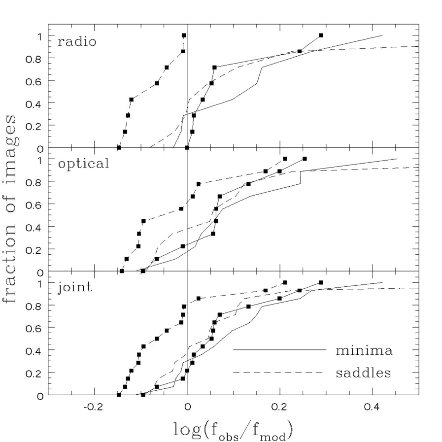Figure B.61. Saddle point suppression in lenses. The three panels show the cumulative distributions of model flux residuals, log(fobs / fmod), in the real data, assuming constant fractional flux errors for each image. The solid (dashed) lines are for minima (saddle points), with squares (no squares) for the distribution corresponding to the most (least) magnified image. From top to bottom the distributions are shown for samples of 8 radio, 10 optical or 15 total four-image lenses. If the flux residuals are created by propagation effects we would not expect the distributions to depend on the image parity or magnification, while if they are due to low optical depth substructure we would expect the distribution for the brightest saddle points to be shifted to lower observed fluxes.

Even though simple Taylor series arguments make it unlikely that changes to the central potential are a solution (see Section B.4.4), it still has its advocates (Evans & Witt [2003], Quadri et al. [2003], Möller, Hewitt & Blain [2003], Kawano et al. [2004]). The basic answer is that it is possible to create flux anomalies by making the deviations of the central potential from ellipsoidal sufficiently large for the angular structure of the potential to change rapidly enough between nearby images to produce the necessary magnification changes. There are three basic problems with this solution (see Section B.4.6 as well).

The first problem is that the required deviations from an ellipsoidal profile far too large. This is true even though the biggest survey of such models allowed image positions to shift by approximately 10 times their actual uncertainties in order to alter the image fluxes (Evans & Witt [2003]) - had they forced the models to match the true astrometric uncertainties they would have needed even larger perturbations. Kochanek & Dalal ([2004]) found that models fitting the flux anomalies required | a₄| >> 0.01 compared to the typical values observed for galaxies and simulated halos | a₄| ~ 0.01 (see Section B.4.4). It is fair to say, however, that the quantitative results on the multipole structure of simulated halos are limited.

The second problem is that when we test these solutions in lenses for which we have additional model constraints, the models are forced back toward the standard ellipsoidal models. The basic problem, as Evans & Witt ([2003]) show, is that the problem of fitting image positions and fluxes with potentials of the form r F() can be reduced a a problem in linear algebra if F() is expanded as a multipole series - by adding enough terms it is possible to fit any four-image lens exactly. The reasons go back to the lack of constraints we discussed in Section B.4.6. Fig B.27 illustrates this point using the lens B1933+503. Kochanek & Dalal ([2004]) first fit the four compact images with a model including deviations from an ellipsoidal surface density. With sufficiently strong deviations there were models that could eliminate the flux anomalies in this system. However, this lens, B1933+503, actually has three components to its source - a compact core forming the four-image system with the anomaly but also to radio lobes lensed into another four-image system and a two-image system for 10 images in all (Fig. B.7). When we add the constraints from these other images the model is forced back to being a standard ellipsoidal model with a flux ratio anomaly. In the future, the degree to which lens galaxy potentials are ellipsoidal could be thoroughly tested in the lenses with Einstein ring images of their host galaxies.

The third problem with using the central potential to produce flux ratio anomalies is that it does not lead to the discrimination between saddle points and minima shown in Fig. B.61. Kochanek & Dalal ([2004]) demonstrate this with Monte Carlo simulations, but the basic reason is simple. Consider a lens like PG1115+080 with two images merging at a saddle point. The sense with which the saddle point and minima are perturbed depends on the phase of the higher order multipoles relative to the images and the critical line, but for any fixed lens potential, that phase varies depending on the source position, so the average effect cannot make the bright saddle points show a significantly different set of properties from the bright minima. Every observed flux anomaly could be explained by adding complex angular structures to the main lens, but the inability of these models to differentiate between saddle points and minima would still rule them out.

For the moment there are two barriers to improving estimates of the substructure mass fraction. First, radio lens surveys have run out of sources bright enough to conduct efficient surveys. This will only change as upgrades to existing radio arrays are completed. The proposed Merlin and VLA upgrades will provide both sensitivity and resolution improvements that will make the next generation of radio lens surveys easier than the last. Second, searches for substructure using optical quasars need to separate the effects of microlensing and substructure. With simple imaging this can be done by finding parts of the quasar which are sufficiently extended to avoid significant contamination from microlensing. Emission line (e.g. Moustakas & Metcalf [2003]) and dust emission regions should both be large enough to filter out the effects of the stars. Studying emission line ratios is now relatively easy because of the new generation of small-pixel integral field spectrographs on 8m-class telescopes. Mid-infrared flux ratios for the dusty regions remain difficult, but the have been obtained for one lens (Q2237+0305, Agol et al. [2000]) and could be extended to several more.

The gold standard, however, would be astrometric detection of dark substructure so that we would obtain a direct, mass estimate. In all the present analyses, the most massive substructures were included as part of the model. They were not, however, dark substructures because they matched to satellites visible in HST images of the lenses. For example, Object X in MG0414+0534 (Fig. B.6) has effects on the image positions that are virtually impossible to reproduce with changes in the potential of the central lens galaxy (Trotter, Winn & Hewitt [2000]), while models with it easily fit the data (Ros et al. [2000]). Fig. B.62 shows the dependence of the goodness of fit to MG0414+0534 on the location of an additional lens component, with a deep minimum located at the observed position of Object X. The deflections produced by an object of mass M generally scale as M^1/2, so it is relatively easy to detect the deflection perturbations from objects only 1% the mass of the primary lens. One approach is to search lenses with VLBI structures for signs of perturbations. This has been attempted for B1152+199 by Metcalf ([2002]), but the case for substructure is not very solid given the limited nature of the data. The cleanest example of astrometric detection of something small, but sadly not dark, is in the VLBI structure of image C in MG2016+112 (Koopmans et al. [2002]). The asymmetry in the VLBI component separations of image C on either side of the critical line (see Fig. B.63) is due to a very faint galaxy 0."8 South of the image with a deflection scale ~ 10% of the primary lens (see Fig. B.6). This is in reasonable agreement with the prediction from the H-band magnitude difference of 4.6 mag and the (lens) Faber-Jackson relation between magnitudes and deflections. In this case, we even know that the satellite is at the same redshift as the lens because Koopmans & Treu ([2002]) accidentally measured its redshift in the course of their observations to measure the velocity dispersion of the lens galaxy.

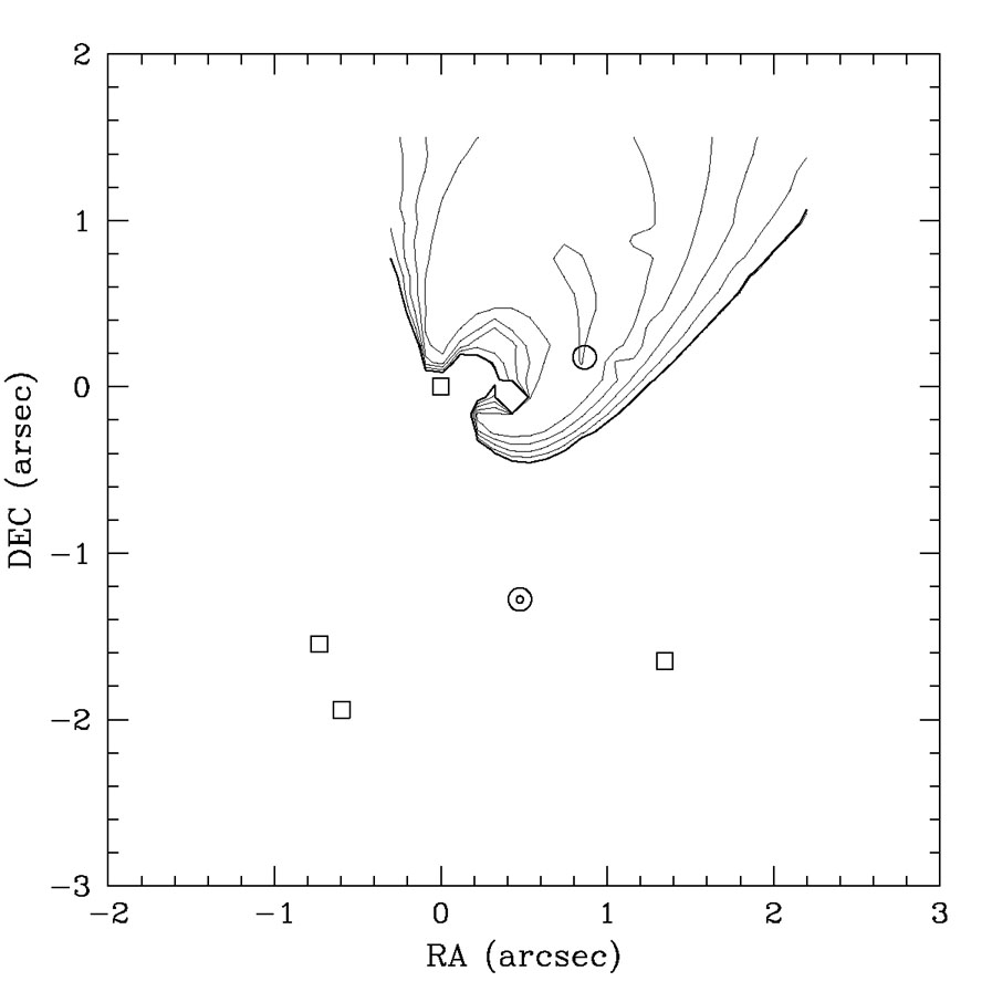Figure B.62. The improvement in the fit to the Ros et al. ([2000]) VLBI data on MG0414+0534 from adding an additional lens with a Einstein radius 15% that of the primary lens galaxy as a function of its position. The squares show the location of the quasar images, the central circles mark the position of the main lens galaxy and the single circle marks the position of object X (see Fig. B.6). The heavy contour has the same 2 = 123 as single component models, and they then drop a factor of 0.2 per lighter contour to a minimum of 2 = 0.6 almost exactly at the position of Object X.

Figure B.63. VLBI maps of MG2016+112 (Koopmans et al. [2002]). The large difference in the C11 / C12 separation as compared to the C13 / C2 separation is the clearest example of an "astrometric" anomaly in a lens. The critical line passes between C12 and C13 and by symmetry we would expect the separations of the subcomponents on either side of the critical line to be similar. In this case the cause of the asymmetry seems to be a galaxy D about 0."8 South of the C image (see Fig. B.6). Galaxy D has the same redshift as the primary lens (Koopmans & Treu [2002]).

⁸ In specific models there can also be global invariants relating image positions and magnifications (e.g. Witt & Mao [2000], Hunter & Evans [2001], Evans & Hunter [2002]). These results are usually for simple softened power law models using either ellipsoidal potentials or an external shear rather than ellipsoidal cuspy density distributions with an external shear, so their applicability to the observed lenses is unclear. Back.

⁹ This is the tidal truncation radius for an SIS of critical radius b orbiting in an SIS of critical radius b₀ > b. The total satellite mass is ab _c. Back.