B.5.3. Observing Time Delays and Time Delay Lenses

The first time delay measurement, for the gravitational lens Q0957+561, was reported in 1984 (Florentin-Nielsen [1984]). Unfortunately, a controversy then developed between a short delay ( 1.1 years, Schild & Cholfin [1986]; Vanderriest et al. [1989]) and a long delay ( 1.5 years, Press, Rybicki, & Hewitt [1992a], [1992b]), which was finally settled in favor of the short delay only after 5 more years of effort (Kundic et al. [1997]; also Schild & Thomson [1997] and Haarsma et al. [1999]). Factors contributing to the intervening difficulties included the small amplitude of the variations, systematic effects, which, with hindsight, appear to be due to microlensing and scheduling difficulties (both technical and sociological).

While the long-running controversy over Q0957+561 led to poor publicity for the measurement of time delays, it allowed the community to come to an understanding of the systematic problems in measuring time delays, and to develop a broad range of methods for reliably determining time delays from typical data. Only the sociological problem of conducting large monitoring projects remains as an impediment to the measurement of time delays in large numbers. Even these are slowly being overcome, with the result that the last five years have seen the publication of time delays in 11 systems (see Table B.5.2).

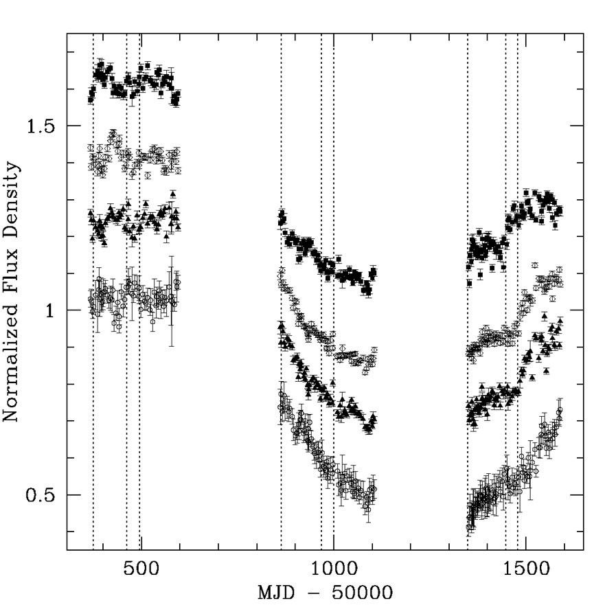
The basic procedures for measuring a time delay are simple. A monitoring campaign must produce light curves for the individual lensed images that are well sampled compared to the time delays. During this period, the source quasar in the lens must have measurable brightness fluctuations on time scales shorter than the monitoring period. The resulting light curves are cross correlated by one or more methods to measure the delays and their uncertainties (e.g., Press et al. [1992a] [1992b]; Beskin & Oknyanskij [1995]; Pelt et al. [1996]; references in Table 1.1). Care must be taken because there can be sources of uncorrelated variability between the images due to systematic errors in the photometry and real effects such as microlensing of the individual images (e.g., Koopmans et al. [2000]; Burud et al. [2002b]; Schechter et al. [2003]). Figure B.35 shows an example, the beautiful light curves from the radio lens B1608+656 by Fassnacht et al. ([2002]), where the variations of all four lensed images have been traced for over three years. One of the 11 systems, B1422+231, is limited by systematic uncertainties in the delay measurements.

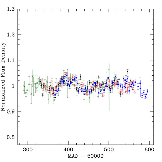Figure B.35. VLA monitoring data for the four-image lens B1608+656. The top panel shows (from top to bottom) the normalized light curves for the B (filled squares), A (open diamonds), C (filled triangles) and D (open circles) images as a function of the mean Julian day. The bottom panel shows the composite light curve for the first monitoring season after cross correlating the light curves to determine the time delays (tAB = 31.5 ± 1.5, tCB = 36.0 ± 1.5 and tDB = 77.0 ± 1.5 days) and the flux ratios. (From Fassnacht et al. [2002].)

We want to have uncertainties in the time delay measurements that are unimportant for the estimates of H₀. For the present, uncertainties of order 3%-5% are adequate (so improved delays are still needed for PG1115+080, HE2149-2745, and PKS1830-211). In a four-image lens we can measure three independent time delays, and the dimensionless ratios of these delays provide additional constraints on the lens models (see Section B.5.1). These ratios are well measured in B1608+656 (Fassnacht et al. [2002]), poorly measured in PG1115+080 (Barkana [1997]; Schechter et al. [1997]; Chartas [2003]) and unmeasured in either RXJ0911+0551 or B1422+231. Using the time delay lenses as very precise probes of H₀, dark matter and cosmology will eventually require still smaller delay uncertainties (~ 1%). Once a delay is known to 5%, it is relatively easy to reduce the uncertainties further because we can accurately predict when flux variations will appear in the other images and the lens will need to be monitored more intensively.

The expression for the time delay in an SIS lens (Eqn. B.94) reveals the other data that are necessary to interpret time delays. First, the source and lens redshifts are needed to compute the distance factors that set the scale of the time delays. Fortunately, we know both redshifts for all 11 systems in Table B.5.2 even though missing redshifts are a problem for the lens sample as a whole (see Section B.2). The dependence of the distances D_d, D_s and D_ds on the cosmological model is unimportant until our total uncertainties approach 5%. Second, we require accurate relative positions for the images and the lens galaxy. These uncertainties are always dominated by the position of the lens galaxy relative to the images. For most of the lenses in Table B.5.2, observations with radio interferometers (VLA, Merlin, VLBA) and HST have measured the relative positions of the images and lenses to accuracies 0."005. Sufficiently deep HST images can obtain the necessary data for almost any lens, but dust in the lens galaxy (as seen in B1600+434 and B1608+656) can limit the accuracy of the measurement even in a very deep image. For B0218+357 and PKS1830-211, however, the position of the lens galaxy relative to the images is not known to sufficient precision or determined only from models (see Biggs et al. [1999], Léhar et al. [2000]; Courbin et al. [2002]; Winn et al. [2002b], Wucknitz, Biggs & Browne [2004], York et al. [2004]).

We can also divide the systems by the complexity of the required lens model. We define eight of the lenses as "simple," in the sense that the available data suggests that a model consisting of a single primary lens in a perturbing shear (tidal gravity) field should be an adequate representation of the gravitational potential. In some of these cases, an external potential representing a nearby galaxy or parent group will improve the fits, but the differences between the tidal model and the more complicated perturbing potential are small (see Section B.5.2). If we neglect the convergence produced by the group, then H₀ may be overestimated. We include the quotation marks because the classification is based on an impression of the systems from the available data and models. Remember also that there are convergence fluctuations along the line of sight that add a low level of cosmic variance to the time delays of individual lenses (Section B.4.2 and Fig. B.19). While we cannot guarantee that a system is simple, we can easily recognize two complications that will require more complex models.

The first complication is that some primary lenses have less massive satellite galaxies inside or near their Einstein rings. This includes two of the time delay lenses, RXJ0911+0551 and B1608+656. RXJ0911+0551 could simply be a projection effect, since neither lens galaxy shows irregular isophotes. Here the implication for models may simply be the need to include all the parameters (mass, position, ellipticity ^... ) required to describe the second lens galaxy, and with more parameters we would expect greater uncertainties in H₀. In B1608+656, however, the lens galaxies show the disturbed isophotes of dusty galaxies possibly undergoing a disruptive interaction. How one should model such a system is unclear. If there was once dark matter associated with each of the galaxies, how is it distributed now? Is it still associated with the individual galaxies? Has it settled into an equilibrium configuration? While B1608+656 can be well fit with standard lens models (Fassnacht et al. [2002], Koopmans et al. [2003]), these complications have yet to be explored in detail.

The second complication occurs when the primary lens is a member of a more massive (X-ray) cluster, as in the time delay lenses RXJ0911+0551 (Morgan et al. [2001]) and Q0957+561 (Chartas et al. [2002]). The cluster model is critical to interpreting these systems (see Section B.5.2). The cluster surface density at the position of the lens (_c 0.2) leads to large corrections to the time delay estimates and the higher-order perturbations are crucial to obtaining a good model. For example, models in which the Q0957+561 cluster was treated simply as an external shear were grossly incorrect (see Section B.4.6, Keeton et al. [2000]). In addition to the uncertainties in the cluster model itself, we must also decide how to include and model the other cluster galaxies near the primary lens. Thus, lenses in clusters have many reasonable degrees of freedom beyond those of the "simple" lenses.