B.6.6. Magnification Bias

The optical depth calculation suggests that the likelihood of finding that a z_s 2 quasar is lensed is very small ( ~ 10^-4) , while observational surveys of bright quasars typically find that of order 1% of bright quasars are lensed. The origin of the discrepancy is the effect known as "magnification bias" (Turner [1980]), which is really the correction needed to account for the selection of survey targets from flux limited samples. Multiple imaging always magnifies the source, so lensed sources are brighter than the population from which they are drawn. For example, the mean magnification of all multiply imaged systems is simply the area over which we observe the lensed images divided by the area inside the caustic producing multiple images because the magnification is the Jacobean relating area on the image and source planes, d² = |µ|^-1 d² . For example, an SIS lens with Einstein radius b produces multiple images over a region of radius b on the source plane (i.e. the cross section is b²), and these images are observed over a region of radius 2b on the image plane, so the mean multiple-image magnification is <µ> = (4 b²) / ( b²) = 4.

Since fainter sources are almost always more numerous than brighter sources, magnification bias almost always increases your chances of finding a lens. The simplest example is to imagine a lens which always produces the same magnification µ applied to a population with number counts N(F) with flux F. The number counts of the lensed population are then N_lens(F) = µ^-1 N(F / µ), so the fraction lensed objects (at flux F) is larger than the number expected from the optical depth if fainter objects are more numerous than the magnification times the density of brighter objects. Where did the extra factor of magnification come from? It has to be there to conserve the total number of sources or equivalently the area on the source and lens planes - you can always check your expression for the magnification bias by computing the number counts of lenses and checking to make sure that the total number of lenses equals the total number of sources if the optical depth is unity.

Real lenses do not produce unique magnifications, so it is necessary to work out the magnification probability distribution P( > µ) (the probability of a magnification larger than µ) or its differential dP / dµ and then convolve it with the source counts. Equivalently we can define a magnification dependent cross section, d / d µ = dP / d µ where is the total cross section. We can do this easily only for the SIS lens, where a source at produces two images with a total magnification of µ = 2 / with µ > 2 in the multiple image region (Eqns B.21, B.22), to find that P( > µ) = (2 / µ)² and dP / dµ = 8 / µ³. The structure at low magnification depends on the lens model, but all sensible lens models have P( > µ) µ^-2 at high magnification because this is generic to the statistics of fold caustics (Part 1, Blandford & Narayan [1986]).

Usually people have defined a magnification bias factor B(F) for sources of flux F so that the probability p(F) of finding a lens with flux F is related to the optical depth by p(F) = B(F). The magnification bias factor is

(B.115)

for a source with flux F, or

(B.116)

for a source of magnitude m. Note the vanishing of the extra 1 / µ factor when using logarithmic number counts N(m) for the sources rather than the flux counts N(F). Most standard models have magnification probability distributions similar to the SIS model, with P( > µ) (µ₀ / µ)² for µ > µ₀, in which case the magnification bias factor for sources with power law number counts N(F) = dN / dF F^- is

(B.117)

provided the number counts are sufficiently shallow ( < 3). For number counts as a function of magnitude N(m) = dN / dm 10^am (where a = 0.4( - 1)) the bias factor is

(B.118)

The steeper the number counts and the brighter the source is relative to any break between a steep slope and a shallow slope, the greater the magnification bias. For radio sources a simple power law model suffices, with 2.07 ± 0.11 for the CLASS survey (Rusin & Tegmark [2001]), leading to a magnification bias factor of B 5. For quasars, however, the bright quasars have number counts steeper than this critical slope, so the location of the break from the steep slope of the bright quasars to the shallower slope for fainter quasars near B ~ 19 mag is critical to determining the magnification bias. Fig. B.45 shows an example of a typical quasar number counts distribution as compared to several (old) models for the distribution of lensed quasars. The changes in the magnification bias with magnitude are visible as the varying ratio between the lensed and unlensed counts, with a much smaller ratio for bright quasars (high magnification bias) than for faint quasars (low magnification bias) and a smooth shift between the two limits as you approach the break in the slope of the counts at B ~ 19 mag.

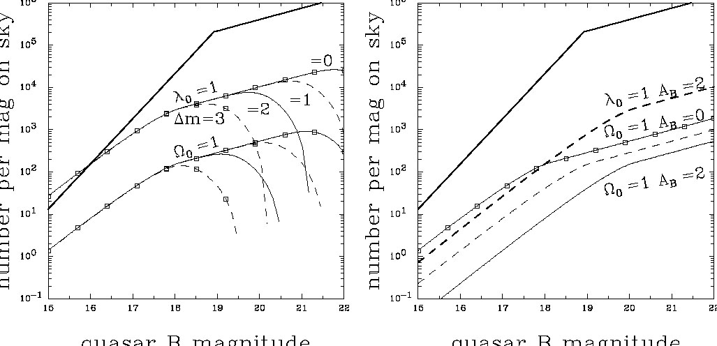Figure B.45. Examples of selection effects on optically selected lens samples. The heavy solid curves in the two panels shows a model for the magnitude distribution of optically-selected quasars. The light curves labeled M = 1 and 0 = 1 show the distribution of lensed quasars for flat cosmologies that are either pure matter or pure cosmological constant. The change in the ratio between the lensed curves and the unlensed curves illustrates the higher magnification bias for bright quasars where the number count distribution is steeper than for faint quasars. In the left panel the truncated curves show the effect of losing the lensed systems where the lens galaxy is m = 1, 2 or 3 magnitudes fainter than the quasars. Once surveys are searching for lensed quasars with B 20 mag, the light from the lens galaxy becomes an increasing problem, particularly since the systems with the brightest lens galaxies will also have the largest image separations that would otherwise make them easily detected. In the left panel we illustrate the effect of adding a net extinction of AB = 1 or 2 mag from dust in the lens galaxies. These correspond to larger than expected color excesses of E(B - V) 0.2 and 0.4 mag respectively. Note how the extinction "undoes" the magnification bias by shifting the lensed distributions to fainter magnitudes.

For optically-selected lenses, magnification bias is "undone" by extinction in the lens galaxy because extinction provides an effect that makes lensed quasars dimmer than their unlensed counterparts. Since the quasar samples were typically selected at blue wavelengths, the rest wavelength corresponding to the quasar selection band at the redshift of the lens galaxy where it encounters the dust is similar to the U-band. If we use a standard color excess E(B - V) for the amount of dust, then the images become fainter by of order A_U E(B - V) magnitudes where A_U 4.9. Thus, if lenses had an average extinction of only E(B - V) 0.05 mag, the net magnification of the lensed images would be reduced by about 25%. If all lenses had the same demagnification factor f < 1 then the modifications to the magnification bias would be straight forward. For power-law number counts N(F) F^-, the magnification bias is reduced by the factor f and a E(B - V) = 0.05 extinction leads to a 50% reduction in the magnification bias for objects with a slope 2 (faint quasars) and to still larger reductions for bright quasars. Some examples of the changes with the addition of a simple mean extinction are shown in the right panel of Fig. B.45, although the levels of extinction shown there are larger than observed in typical lenses as we discuss in Section B.9.1. Comparisons between the statistics of optically-selected and radio-selected samples can be used to estimate the magnitude of the correction. The only such comparison found estimated extinctions consistent with the direct measurements of Section B.9.1 (Falco, Kochanek & Muñoz [1998]). However, the ISM of real lenses is presumably far more complicated, with a distribution of extinctions and different extinctions for different images which may be a function of orientation and impact parameter relative to the lens galaxy, for which we have no good theoretical model.

The flux of the lens galaxy also can modify the magnification bias for faint quasars, although the actual sense of the effect is complex. The left panel Fig. B.45 shows the effect of dropping lenses in which the lens galaxy represents some fraction of the total flux of the lensed images. The correction is unimportant for bright quasars because lens galaxies with B < 19 mag are rare. In this picture, the flux from the lens galaxy leads to the loss of lenses because the added flux from the lens galaxy makes the colors of faint lensed quasars differ from those of unlensed quasars so they are never selected as quasars to begin with. Alternatively, if one need not worry about color contamination, then the lens galaxy increases the magnification bias by supplying extra flux that makes lensed quasars brighter.

Any other selection effect, such as the dynamic range allowed for flux ratios between images as a function of their separation will also have an effect on the magnification bias. Exactly how the effect enters depends on the particular class of images being considered. For example, in the SIS lens (or more generally for two-image lenses), a limitation on the detectable flux ratio 0 < f_min < 1 sets a minimum detectable magnification µ_min = 2(1 + f_min) / (1 - f_min) > µ₀ = 2. Since most lens samples have significant magnification bias, which means that most lenses are significantly magnified, such flux limits have only modest effects. The other limit, which cannot be captured in the SIS model, is that almost all bright images are merging pairs on folds (or triplets on cusps) so the image separation decreases as the magnification increases. The contrast between the merging images and any other images also increases with increasing magnification - combined with limits on the detectability of images, these lead to selection effects against highly magnified images. This is also usually a modest effect - while magnification bias is important, the statistics are dominated by modestly magnified systems rather than very highly magnified images. In fact, there are have been few attempts at complete studies of the complicated interactions between finding quasars, finding lenses, selection effects and magnification bias. There is an early general study by Kochanek ([1991b]) and a detailed practical application of many of these issues to the SDSS survey by Pindor et al. ([2003]). Unfortunately, Pindor et al. ([2003]) seem to arrive at a completeness estimate from their selection model that is too high given the number of lenses they found in practice. Some of this may be due to underestimating the luminosity of lens galaxies, the effects of the lens galaxy or extinction on the selection of quasars or the treatment of extended, multicomponent lenses compared to normal quasars in the photometric pipeline. These difficulties, as well as the larger size of the present radio-selected lens samples, are the reason that almost all recent statistical studies have focused exclusively on radio lenses.

The standard magnification bias expressions (Eqns. B.115 and B.116) are not always appropriate. They are correct for the statistics of lenses selected from source populations for which the total flux of the source (including all images of a lensed source) is defining F (or m). This is true of most existing surveys - for example the CLASS radio survey sources were originally selected from single dish observations with very poor resolution compared to typical image separations (see Browne et al. [2003]). If, however, the separation of the images is large compared to the resolution of the observations and the fluxes of the images are considered separately, then the bias must be computed in terms of the bright image used to select sources to search for additional images. This typically reduces the bias. More subtle effects can also appear. For example, the SDSS survey selects quasar candidates based on the best fit point-source magnitudes, which will tend to be an underestimate of the flux of a resolved lens. Hence the magnification bias for lenses found in the SDSS survey will be less than in the standard theory. Samples selected based on more than one frequency can have more complicated magnification biases depending on the structure of the multidimensional number counts (Borgeest, von Linde & Refsdal [1991], Wyithe, Winn & Rusin [2003]). The exact behavior is complex, but the magnification bias can be tremendously increased if the fluxes in the bands are completely uncorrelated or tightly but nonlinearly correlated. For example, if the luminosities in bands A and B are related by tight, nonlinear correlation of the form L_A L_B^1/2, then the lensed examples of these objects will lie off the correlation. At present, there are too few deep, wide-area multiwavelength catalogs to make good use of this idea, but this is changing rapidly.

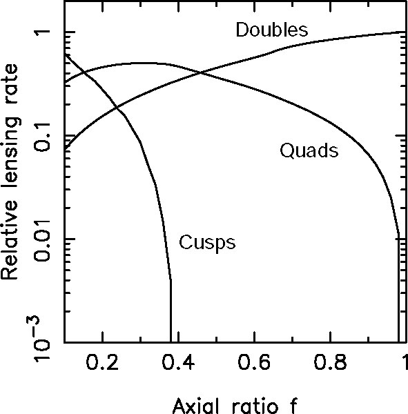
In general, the ellipticity of the lenses has little effect on the expected number of lenses, allowing the use of circular lens models for statistical studies that are uninterested in the morphologies of the images (e.g. Keeton, Kochanek & Seljak [1997], Rusin & Tegmark [2001], Chae [2003]). However, the effects of ellipticity are trivially observable in the relative numbers of two-image and four-image lenses. We noted earlier that the expectation from the cross section is that four-image lenses should represent order ² ~ ² ~ 0.01 of lenses where is the ellipticity of the lens potential. Yet in Section B.2 we saw that four-image lenses represent roughly one third of the observed population. The high abundance of four-image lenses is a consequence of the different magnification biases of the two-image multiplicities - the four-image lenses are more highly magnified than the two-image lenses so they have a larger magnification bias factor.

Fig. B.46 shows the image magnification contours for an SIS lens in an external shear on both the image and source planes. The highly magnified regions are confined to lie near the critical line. If we Taylor expand the inverse magnification radially, then µ^-1 = x| dµ^-1 / dx| where x is the distance from the critical line, so the magnification drops inversely with the distance from the critical line. If we Taylor expand the lens equations, then we find that the change in source plane coordinates is related to the change in image plane coordinates by = µ^-1 x µ^-2. Thus, if L is the length of the astroid curve, the probability of a magnification larger than µ scales as P( > µ) µ^-2L / | dµ^-1 / dx|. This applies only to the four image region, because the only way to get a high magnification in the two-image region is for the source to lie just outside the tip of a cusp. The algebra is overly complex to present, but the generic result is that the region producing magnification µ extends µ^-2 from the cusp tip but has a width that scales as µ^-1/2, leading to an overall scaling that the asymptotic cross section declines as P( > µ) µ^-7/2 rather than P( > µ) µ^-2. This can all be done formally (see Blandford & Narayan [1986]) so that asymptotic cross sections can be derived for any model (e.g. Kochanek & Blandford [1987], Finch et al. [2002]), but a reasonable approximation for the four-image region is to compute the magnification, µ₀, for the cruciform lens formed when the source is directly behind the lens and then use the estimate that P( > µ) = (µ₀ / µ)². Unfortunately, such simple estimates are not feasible for the two-image region. These distributions are relatively easy to compute numerically, as in the example shown in Fig. B.47.

Figure B.46. Magnification contours on the image (left) and source (right) planes for an SIS in an external shear. The heavy solid contours show the tangential critical line (left) and its corresponding caustic (right). On the image plane (left), the light curves are magnification contours. These are positive outside the critical curve and negative inside the critical curve. The images found in a four-image lens are all found in the region between the two dashed contours - when two images are merging on the critical line, the other two images lie on these curves. On the source plane the solid (dashed) curves show the projections of the positive (negative) magnification contours onto the source plane. Note that the high magnification regions are dominated by the four-image systems with the exception of the small high magnification regions found just outside the tip of each cusp.

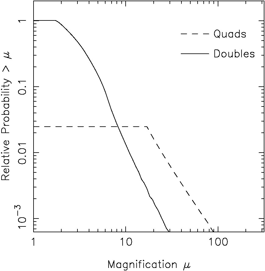Figure B.47. The integral magnification probability distributions for a singular isothermal ellipsoid with an axis ratio of q = 0.7 normalized by the total cross section for finding two images. Note that the total four-image cross section is only of order 2 ~ ( / 3)2 ~ 0.01 of the total, but that the minimum magnification for the four-image systems (µmin ~ 1 / ~ 10) is much larger than that for the two-image systems (µmin ~ 2 just as for an SIS). The entire four-image probability distribution is well approximated by the P( > µ) µ-2 power law expected for fold caustics, while the two-image probability distribution is steeper since highly magnified images can only be created by the cusps. Figure courtesy of D. Rusin. Figure B.48. The expected number of two-image, four-image and three-image (disk or cusp) lenses as a function of axis ratio f for the CLASS sample. From Rusin & Tegmark ([2001]).

Because the minimum magnification of a four-image lens increases µ₀ ^-1 even as the cross section decreases as ₄ ², the expected number of four-image lenses in a sample varies much more slowly with ellipticity than expected from the cross section. The product ₄ B(F) ² µ₀^-1, of the four-image cross section, ₄, and the magnification bias, B(F), scales as ^3- for the CLASS survey ( 2), which is a much more gentle dependence on ellipticity than the quadratic variation expected from the cross section. There is a limit, however, to the fraction of four-image lenses. If the potential becomes too flat, the astroid caustic extends outside the radial caustic (Fig. B.18), to produce three-image systems in the "disk" geometry rather than additional four-image lenses. In the limit that the axis ratio goes to zero (the lens becomes a line), only the disk geometry is produced. The existence of a maximum four-image lens fraction, and its location at an axis ratio inconsistent with the observed axis ratios of the dominant early-type lenses has made it difficult to explain the observed fraction of four image lenses (King & Browne [1996], Kochanek [1996b], Keeton, Kochanek & Seljak [1997], Keeton & Kochanek [1998], Rusin & Tegmark [2001]). Recently, Cohn & Kochanek ([2001]) argued that satellite galaxies of the lenses provide the explanation by somewhat boosting the fraction of four-image lenses while at the same time explaining the existence of the more complex lenses like B1359+154 (Myers et al. [1999], Rusin et al. [2001]) and PMNJ0134-0931 (Winn et al. [2002c], Keeton & Winn [2003]) formed by having multiple lens galaxies with more complex caustic structures. It is not, however, clear in the existing data that four-image systems are more likely to have satellites to the lens galaxy than two-image systems as one would expect for this explanation.

Gravitational lenses can produce highly magnified images without multiple images only if they are highly elliptical or have a low central density. The SIS lens has a single-image magnification probability distribution of dP / dµ = 2 b² / (µ - 1)³ with µ < 2 compared to dP / dµ = 2 b² / µ³ with µ 2 for the multiply imaged region, so single images are never magnified by more than a factor of 2. For galaxies, where we always expect high central densities, the only way to get highly magnified single images is when the astroid caustic extends outside the radial caustic (Fig. B.18). A source just outside an exposed cusp tip can be highly magnified with a magnification probability distribution dP / dµ µ^-7/2. Such single image magnifications have recently been a concern for the luminosity function of high redshift quasars (e.g. Wyithe [2004], Keeton, Kuhlen & Haiman [2004]) and will be the high magnification tail of any magnification perturbations to supernova fluxes (e.g. Dalal et al. [2003]). As a general rule for galaxies, the probability of a single image being magnified by more than a factor of two is comparable to the probability of being multiply imaged.