


B.6.8. The Current State
Recent analyses of lens statistics have focused exclusively on the CLASS flat spectrum radio survey (Browne et al. [2003]). Chae et al. ([2002]), Chae ([2003]) and Mitchell et al. ([2004]) focus on estimating the cosmological model and find results in general agreement with estimates from Type Ia supernovae (e.g. Riess et al. [2004]). The general approach of both groups is to use variants of the maximum likelihood methods described above in Section B.6.7. Chae ([2003]) uses an obsolete estimate of the galaxy luminosity function combined with a Faber-Jackson relation and the variable transformation of Eqn. B.103 but normalized the velocity scale using the observed distribution of lens separations. Mitchell et al. ([2004]) use the true velocity dispersion function from the SDSS survey (Sheth et al. [2003]) and incorporate a Press-Schechter ([1974]) model for the evolution of the velocity function. Chae ([2003]) used ellipsoidal galaxies, although this has little cosmological effect, while Mitchell et al. ([2004]) considered only SIS models. Fig. B.49 shows the cosmological limits from Mitchell et al. ([2004]), which are typical of the recent results . There are also attempts to use lens statistics to constrain dark energy (e.g. Chae et al. [2004], Kuhlen, Keeton & Madau [2004]), but far larger, well-defined samples are needed before the resulting constraints will become interesting.
 |
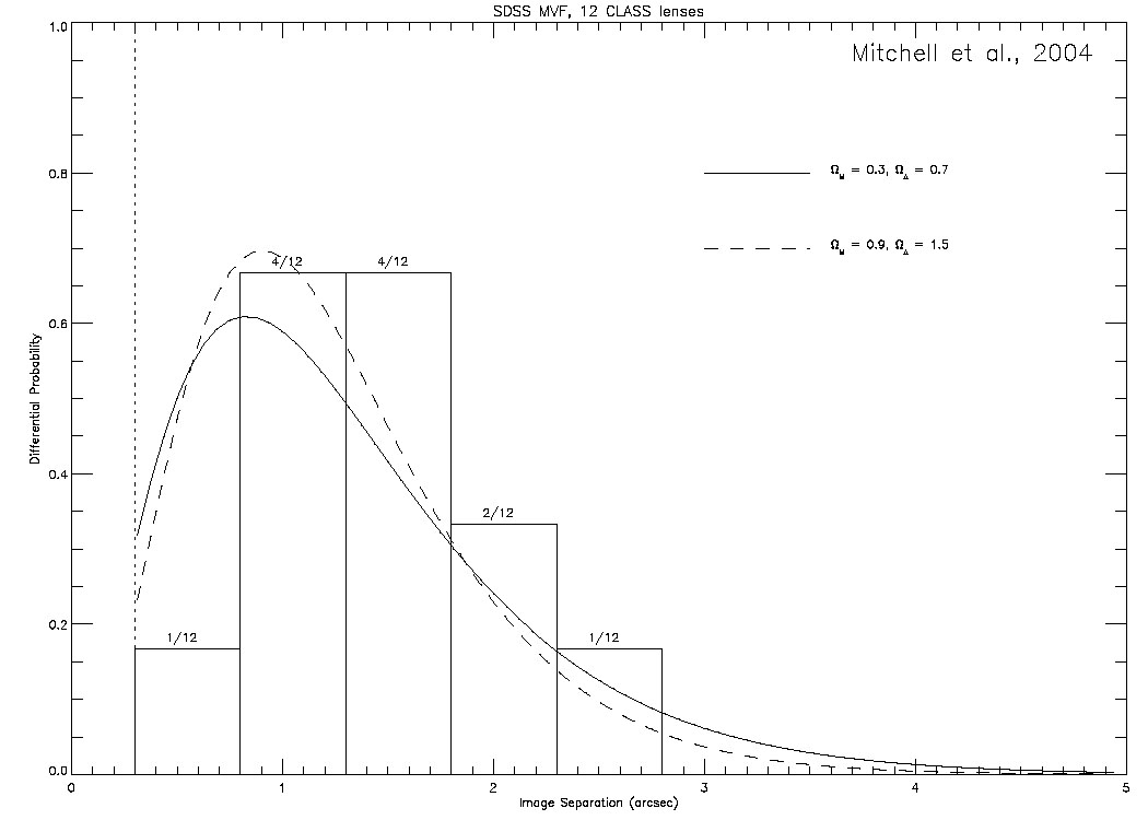 |
Figure B.49. (Top) Likelihood functions for the cosmological model from Mitchell et al. ([2004]) using the velocity function of galaxies measured from the SDSS survey and a sample of 12 CLASS lenses. The contours show the 68, 90, 95 and 99% confidence intervals on the cosmological model. In the shaded regions the cosmological distances either become imaginary or there is no big bang. (Bottom) The histogram shows the separation distribution of the 12 CLASS lenses used in the analysis and the curve shows the distribution predicted by the maximum likelihood model including selection effects. |
Chae & Mao
([2003]),
Davis, Huterer & Krauss
([2003])
and Ofek, Rix & Maoz
([2003])
focused on galaxy properties
and evolution in a fixed, concordance cosmology rather than on determining
the cosmological models. Mitchell et al.
([2004])
compared
models where the lenses evolved following the predictions of CDM models in
comparison to non-evolving models. Because lens statistical estimates
are unlikely
to complete with other means of estimating the cosmological models, these
are more promising applications of gravitational lens statistics for
the future. Attempts to estimate the evolution of the lens population
usually allow the n* and
 *
parameters of the velocity function
(Eqn. B.103) to evolve as power laws with redshift. Mitchell
et al. ([2004],
Fig. B.44) point out that
CDM halo models make specific predictions for the evolution of the velocity
function that have a different structure from simple power laws in
redshift, but with the present data the differences are probably
unimportant. All these evolution studies came to the conclusion that
the number density of the
v ~
*
galaxies which dominate lens statistics has changed little
(
*
parameters of the velocity function
(Eqn. B.103) to evolve as power laws with redshift. Mitchell
et al. ([2004],
Fig. B.44) point out that
CDM halo models make specific predictions for the evolution of the velocity
function that have a different structure from simple power laws in
redshift, but with the present data the differences are probably
unimportant. All these evolution studies came to the conclusion that
the number density of the
v ~
*
galaxies which dominate lens statistics has changed little
( ± 50%)
between the present day and redshift unity.
± 50%)
between the present day and redshift unity.
I have three concerns about these analyses and their focus on the "complete" CLASS lens samples. First, a basic problem with the CLASS survey is that we lack direct measurements of the redshift distribution of the source population forming the lenses (e.g Marlow et al. [2000], Muñoz et al. [2003]). In particular, Muñoz et al. ([2003]) note that the radio source population is changing radically from nearly all quasars to mostly galaxies as you approach the fluxes of the CLASS source population. This makes it dangerous to extrapolate the source population redshifts from the brighter radio fluxes where the redshift samples are nearly complete to the fainter samples where they are not. The second problem is that no study has a satisfactory treatment of the lenses with satellites or associated with clusters. All the analyses use isolated lens models and then either include lenses with satellites but ignore the satellites or drop lenses with satellites and ignore the fact that they have been dropped. The analysis by Cohn & Kochanek ([2004]) of lens statistics with satellites shows that neither approach is satisfactory - dropping the satellites biases the results to underestimate cross sections while including them does the reverse. Cohn & Kochanek ([2004]) concluded that including they systems with satellites probably has fewer biases than dropping them. A similar problem probably arises from the effects of the group halos to which many of the lenses belong (e.g. Keeton et al. [2000], Fassnacht & Lubin [2002]). My third concern is that the separations of the radio lenses seen to be systematically smaller than the optically selected lenses even though the optical HST Snapshot survey (Maoz et al. [1993]) had the greatest sensitivity to small separation systems. It is possible that this is simply due to selection effects in the optical samples, but I have seen no convincing scenario for producing such a selection effect. We see no clear correlation of extinction with image separation (see Section B.9.1), emission from the lens galaxy is less important for small separation systems than for large separation systems, and the selection function due to the resolution of the observations is fairly simple to model.
On the other hand, the various lens samples may all consistent. One way to compare the different data sets is to non-parametrically construct the velocity function from the observed image separations of the samples. To do this we assume an SIS lens model for the conversion from image separations to circular velocities, and then adopt the standard non-parametric methods used to construct luminosity functions from redshift surveys to construct the velocity function from the image separations (Kochanek [2003c]). The results for the flat-spectrum lens surveys (CLASS, JVAS, PANELS), all radio surveys and all radio surveys plus the quasar lenses are shown in Fig. B.50. We normalized the estimates to the density at vc = 300 km/s to eliminate any dependence on the cosmological model. The lens data can estimate the velocity function from roughly vc ~ 100 km/s to 500 km/s. At lower velocities the finite resolution of the observations makes the uncertainties in the density explode, and at higher velocities the surveys have not searched large enough angular regions around the lens galaxies. The shape of the velocity function is consistent with local estimates (Fig. B.42) except in the highest circular velocity bin where we begin to see the contribution from clusters we will consider in Section B.7. Fig. B.50 also makes it clear why constraints on the evolution of the lenses are so weak - evolution estimates basically try to compare the low-redshift separation distribution to the high redshift separation distribution, and we simply do not have large enough lens samples to begin subdividing them in redshift (to say nothing of dealing with unmeasured redshifts) and still have small statistical uncertainties.
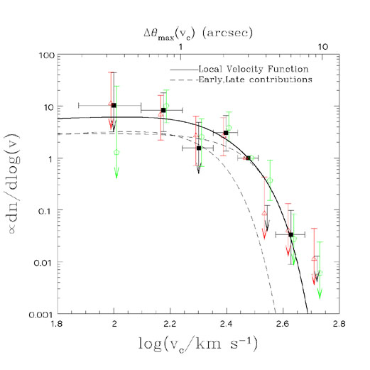 |
Figure B.50. Non-parametric reconstructions of the velocity function from the observed separations of gravitational lenses assuming an SIS lens model. The velocity functions are all normalized to the bin centered at 300 km/s. The filled squares use only the lenses in the flat spectrum radio surveys, the triangles use all radio-selected lenses and the pentagons include all radio lenses and all quasar lenses. The horizontal error bars on the filled squares show the bin widths. The triangles and pentagons are horizontally offset from the squares to make them more visible. The curves show the velocity function estimated from the 2MASS sample from Fig. B.42. The horizontal scale at the top of the figure shows the maximum separation produced by a lens of the corresponding circular velocity. The mean separation produced by such a lens will be one-half the maximum. |