Annu. Rev. Astron. Astrophys. 2011. 49:409-470 Copyright © 2011 by Annual Reviews. All rights reserved

2. THEORETICAL BASIS

This section sketches a theoretical description of the halo framework that supports cluster cosmology. There is considerable richness to the galaxy formation problem that we omit here; the recent review of Benson (2010) provides substantial detail. Simulation studies of halo evolution into the strongly non-linear regime are becoming increasingly powerful, but finite resolution and uncertainty in astrophysical treatments limit predictive power. While not yet robust enough to offer sharp prior characterization of the astrophysics required for cosmological studies, simulations offer key insights into the structure and physics sensitivity of the functions that relate observable signals to halo mass and epoch.

2.1. LSS and Halo Formation from Inflation

Ample evidence now supports the picture that LSS formed via gravitational amplification of initially small density fluctuations, δ ≡ (ρ − ) / . Cosmic microwave background anisotropy measurements are consistent with expectations from a large class of basic inflationary models (e.g., Baumann & Peiris 2009). Such models are characterized by an instantaneous primordial power spectrum, P_prim(k) ∼ | δ_k(a)²| ∼ k^n_s, with spectral index, n_s, expected to be close to unity. Here, δ_k is the Fourier transform of the density fluctuations, δ(x).

After inflation ceases, fluctuations in the coupled photon-baryon-dark matter fluid evolve in ways that are now well understood from linearized Boltzmann treatments (Seljak et al. 2003). For the standard case of adiabatic fluctuations, and on scales above the baryon Jeans mass, the post-recombination matter (dark matter and baryons) power spectrum exhibits a growing mode that scales with the cosmic expansion parameter, a, as

(1)

Here, T(k, θ_Ω) is a transfer function that encapsulates evolution before recombination at z ∼ 1100, G(a, θ_Ω) is the density perturbation growth factor from linear theory, and θ_Ω is the controlling parameter set of the background cosmological model. Dark energy models that involve modifications to general relativity may introduce k-dependence into the growth function above.

The power spectrum in the reference ΛCDM model is set by present-epoch energy densities, θ_Ω = { Ω_b h², Ω_c h², Ω_Λ }, where h = H₀ / 100 km s⁻¹ Mpc⁻¹ is the dimensionless Hubble constant and Ω_X ≡ ρ_X / ρ_cr is the density of component X relative to the critical density, ρ_cr = 3H₀² / 8 π G. The curvature density, 1 − ∑_X Ω_X, is zero to within ± 0.007 (Komatsu et al. 2011), consistent with a flat spatial metric on cosmic scales. Our notation uses ‘b’ for baryons, ‘c’ for cold, dark matter (CDM), and ‘m’ for all matter: Ω_m = Ω_b + Ω_c. In the minimal model, the dark energy is a vacuum energy with equation of state, p = − ρ c². We use Ω_Λ for this case and employ Ω_DE when referring to models wherein the dark energy equation of state, w = p / (ρ c²), differs from −1.

Current constraints for a flat ΛCDM model from CMB measurements, combined with angular clustering of red galaxies and local measurements of H₀, are shown in Table 1 (Komatsu et al. 2011). The parameter Δ²(k) is the variance in density fluctuations evaluated at horizon crossing, which is independent of k for n_s = 1, and the wavenumber k₀ = 0.002 ⁻¹ corresponds to a large comoving length scale, ∼ π / k₀ = 1.6 Gpc.

Table 1. Flat ΛCDM Parameters ^a from WMAP+BAO+H₀

Parameter	Value
ΩΛ	0.725 ± 0.016
Ωc	0.229 ± 0.015
Ωb	0.0458 ± 0.0016
h	0.702 ± 0.014
ns	0.968 ± 0.012
1010 Δ2(k0)	0.2430 ± 0.0091
σ8	0.816 ± 0.024
a From Komatsu et al. (2011).

In the minimal model, the matter density fluctuations filtered within a sphere of comoving radius R are Gaussian distributed with zero mean. The comoving radius defines a mass, M = (4π / 3) ρ_cr R³, of matter within that radius in the young universe, when Ω_m(a) = 1. Early observations that the variance in galaxy counts is near unity on a scale of R = 8 h⁻¹ led to this as a conventional choice of scale at which to quote the fluctuation amplitude (see Table 1). The corresponding mass, M = 0.59 × 10¹⁵ h⁻¹ M_⊙, is characteristic of rich clusters of galaxies.

The variance of linearly-evolved, CDM fluctuations, filtered on mass scale M, has the form

(2)

where the filter function is W(y) = 3[sin(y) / y³ − cos(y) / y²] for the typical case of sharp (or top-hat) spatial filtering within radius R. Evaluating Equation 2 at 8 h⁻¹ and a = 1 produces the oft-quoted matter power spectrum normalization parameter, σ₈. We will see below that σ(M, a) serves as a similarity variable for expressing model-independent forms of the halo space density and clustering.

The evolution of the fluctuation spectrum, Equation 1, is valid at early times or at scales sufficiently large so that σ(M, a) ≪ 1 at all times. On small scales, where CDM power spectra are generically maximum, fluctuation growth produces δ ≥ 1, and linear theory breaks down. Mode-mode coupling terms become important to the dynamics, and solutions in Fourier space become difficult. While higher-order perturbation theory solutions can extend analytic evolution to later times than linear theory (e.g., Bernardeau et al. 2002; Crocce & Scoccimarro 2006), the full problem is typically treated using N-body simulations, discussed below.

A recent analytical advance considers LSS as an effective fluid. Baumann et al. (2010) show that integrating out small-scale, non-linear structures renormalizes the cosmological background and introduces dissipative terms, of order v² / c², into the dynamics of large-scale modes, with v the typical velocity dispersion of collapsed halos. Since even the most massive halos have v < 0.01c, the magnitude of these effects is very small. Furthermore, Baumann et al. (2010) show that virialized halos decouple completely from large-scale dynamics, at all orders in the post-Newtonian expansion.

2.1.1. HALO MODEL DESCRIPTION OF LSS

Astrophysical structures, from the first stars at high redshift to galaxy clusters at low redshift, tend to emerge from local maxima of the filtered density field. While density peaks are generally non-spherical (Bardeen et al. 1986), a first-order description considers them spherical and isolated from their surroundings. Birkhoff's theorem then implies that the expansion histories of radial mass shells within a peak follow trajectories perturbed from the overall background, with sufficiently dense shells expanding to a maximum size and then contracting. The traditional ansatz assumes collapse by a radial factor of two (Gunn & Gott 1972), after which a quasi-virialized and quasi-hydrostatic structure – a perfectly spherical halo – is born.

The collapse criterion is that the linearly-evolved perturbation amplitude reach a critical value, δ(a) = δ_c, with δ_c = 1.686 the conventional choice. Applying this idea to the CDM spectrum, Equation 2, leads to a characteristic mass scale, M_∗(a), defined by σ[M_∗(a), a] = δ_c. At a given epoch, a spectrum of halo masses exist, with masses above (below) M_∗(a) forming from perturbations with amplitudes above (below) the rms level of the filtered Gaussian spectrum. Considerable literature (e.g., Press & Schechter 1974; Bond et al. 1991; Bond & Myers 1996; Sheth & Tormen 1999 and many others) has established this picture as the halo model of large-scale structure. We review here only aspects relevant for cluster cosmology; a more thorough review can be found in Cooray & Sheth (2002).

The basic element of the halo model is the population mean space density, n(M, z), in units of number per unit comoving volume, commonly referred to as the mass function. Expressed as a differential function of mass, it takes the form

(3)

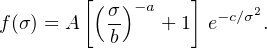
where _m = Ω_m ρ_cr is the comoving mean matter density and f(σ) is a model-dependent function of the filtered perturbation spectrum, Equation 2. Analytic forms for f(σ) capture much, but not all, of the behavior seen in N-body simulations, as discussed below.

The spatial clustering of halos is described by a modified version of the matter power spectrum. On large spatial scales, or low wavenumbers, the halo autocorrelation power spectrum is modified,

(4)

where b(M, a), the halo bias function, is independent of k, for the case of Gaussian fluctuations, but dependent on mass and epoch. While this expression applies to the spatial autocorrelation of systems with fixed mass M, it generalizes to the cross-correlation between sets of halos at different masses, P_h1h2(k, a) = b(M₁, a) b(M₂, a) P_m(k, a). The theory of peaks in Gaussian random fields expresses the bias as a function of the normalized peak height, ν = δ_c / σ(M,a) (Kaiser 1984; Bardeen et al. 1986).

Below, we show that N-body simulations support the forms of equations (3) and (4), but a precise fit to the mass function requires that f(σ) be adjusted to include explicit redshift dependence, f(σ, z). There are subtleties to the definition of mass in simulations that must also be taken into account.

2.1.2. ASTROPHYSICAL PROCESSES

Various astrophysical processes play out within the photon-baryon components of the evolving cosmic web, including hydrodynamic, magnetohydrodynamic and radiative transfer effects; star and black hole formation with associated feedback of momentum, energy and entropy; and so on. Except for the immediate vicinity of black holes, these processes involve classical physics that is largely known. But the fully three-dimensional and non-linear nature of the problem, the wide dynamic range in length and time scales, and the non-trivial couplings among the constituent physical processes introduce tremendous complexity into baryon evolution. Galaxy formation is truly a Grand Challenge computational problem. We touch on select issues relevant to the observable features of galaxy clusters.

Shocks and turbulent MHD heating. During halo formation, gravitational potential energy in the baryonic component is thermalized via shocks. The highest Mach numbers, of tens or more, should occur in the accretion shocks at the edges of clusters (e.g. Pfrommer et al. 2006). While these strong shocks are expected to be efficient particle accelerators, recent observations place tight limits on the volume-averaged pressure contributions from relativistic particles (Ackermann et al. 2010). Shocks with Mach numbers of a few are also associated with major mergers: a spectacular example is the narrow radio relic in the cluster CIZA J2242.8+5301, for which van Weeren et al. (2010) use multi-frequency radio and polarization observations to infer a Mach number 4.6 _−0.9^+1.3 in a shock located 1.5 from the cluster center. Most of the energy thermalized during cluster formation, however, is dissipated in weak shocks that are persistently driven by dissipating sub-structures and ongoing minor mergers. Shocks are also driven by jets from AGNs and, at earlier times, by winds from star forming galaxies.

Details of the nano-parsec scale physics that drive thermalization remain under active study, especially the roles of magnetic fields, turbulence and plasma instabilities (e.g., Kunz et al. 2011). Observations and simulations discussed below indicate that thermalization is efficient; thermal pressure supplies the bulk of support against gravity within the halo potential except during brief periods near periapsis of major mergers.

Radiative cooling. Since the intracluster plasma (and, to a lesser extent, its interstellar counterpart) is optically thin at most wavelengths, radiation loss is the primary cooling mechanism for the baryonic component of halos. Indeed, the classic criterion for setting an upper bound on galaxy size comes from balancing the gas cooling time against the halo dynamical time (White & Rees 1978). The first generation of stars form at z ∼ 30, aided by molecular hydrogen line emission, within halos of mass ∼ 10⁶ M_⊙ (Abel, Bryan & Norman 2002; Bromm et al. 2009). By z ∼ 10, atomic line cooling in halos with virial temperatures above 10⁴ K produces the first generation of galaxies, which grow hierarchically for a time determined by the large-scale environment. Proto-cluster regions have more efficient cooling at high redshift than do proto-voids, but the feedback from vigorous, early production of compact sources helps to quench star formation before a large fraction of baryons are converted to stars.

The cooling timescale of the gas in massive halos is typically longer than a Hubble time, except for a subset of systems that exhibit cool cores. The central ∼ 100 region of such systems tends to be X-ray bright and typically contains a dominant elliptical galaxy. We discuss aspects of cool core phenomenology in Section 6.4.

Star and black hole formation. Cold, molecular gas fuels star formation. The star formation rate can roughly be considered as proportional to the local rate of gas cooling below 10⁴ K, but there are other considerations. Different venues for star formation exist, ranging from quiescent disks to the bulges of tidally-triggered starburst galaxies, and it is not yet clear whether a single model based on local gas conditions captures the full range of observed behavior. Supermassive black hole (SMBH) growth occurs through mergers and accretion in galactic cores, and these central engines drive quasar and radio jet activity (e.g., Di Matteo, Springel & Hernquist 2005). Sloan Digital Sky Survey (SDSS) quasar studies indicate that SMBHs of mass ∼ 10⁹ M_⊙ exist at z = 7 (Fan 2006), and processes for forming such large black holes in the first few hundred million years of the universe have been proposed (Volonteri 2010).

In Gaussian random fields, small-scale peaks are more abundant when embedded within large-scale peaks, so the largest galaxies and quasars at high redshift represent the progenitors of massive galaxies observed in low redshift clusters.

Feedback from compact sources. Feedback of mass, momentum, and entropy from stellar/SMBH sources is important at all stages of the LSS hierarchy. Photoionization and supernova-driven winds serve to limit cooling and star formation in low-mass halos (Dekel & Silk 1986). Jets driven by accretion onto the central SMBH appear to be required to limit the maximum size of galaxies (e.g., Croton et al. 2006; Cattaneo et al. 2009). Formulations for this feedback typically tie the energy input to the mass accretion rate which, in turn, is governed by the local rate of cooling and/or cold accretion.

The end result of this competition between cooling and heating is that heating largely wins. The overall efficiency of star formation is small, and peaks in halos of roughly galactic scale (e.g. Moster et al. 2010). Figure 2 shows a recent compilation of stellar mass fraction (M_star / M) measurements as a function of halo circular velocity, v_circ = √GM / r, with M the total halo mass and r its radius (Dai et al. 2010). The horizontal lines show the cosmic baryon fraction, Ω_b / Ω_m = 0.171 ± 0.009, derived from Wilkinson Microwave Anisotropy Probe (WMAP) data analysis (Dunkley et al. 2009).

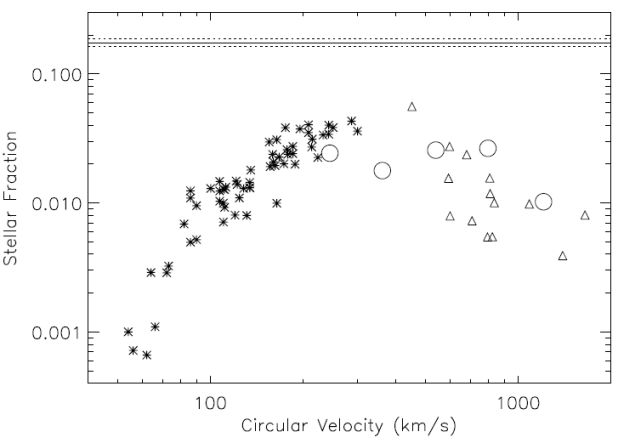Figure 2. The observed stellar mass fraction as a function of halo circular velocity for systems ranging from galaxies to rich clusters indicates that star formation efficiency peaks in halos of mass ∼ 1013 h−1 M⊙. From Dai et al. (2010).

Minor mergers, while much more frequent, are also less damaging. Current simulations and observations indicate that the dynamical and thermodynamical response of halos is quite fast. Hydrostatic and virial equilibrium assumptions are typically valid to within roughly ten percent for the majority of the cluster population (e.g. Rasia et al. 2006; Nagai, Vikhlinin & Kravtsov 2007).

All this astrophysical evolution offers a treasure trove of observational possibilities. Uniquely in massive clusters, all of the matter is readily observed, allowing a complete census to be taken. Stars make up 1–3% (Lin & Mohr 2004; Gonzalez, Zaritsky & Zabludoff 2007; Giodini et al. 2009); ∼ 15% resides in the hot, diffuse, intergalactic gas (Allen et al. 2008; Simionescu et al. 2011); and the rest is in the form of non-baryonic CDM (Section 5.1).

2.2. Cosmological Tests with Massive Halos

As tracers of massive halos, galaxy clusters provide a number of signatures that are sensitive to the underlying cosmology. We review here the principles underlying key methods. A typical set of cosmological parameters for such studies might consist of the primordial spectrum amplitude and slope, the present-epoch densities of the three energy components dominant at late times, the dimensionless Hubble constant, and the DE equation of state parameters,

(5)

where the last two parameters define a linearly-evolving DE equation of state,

(6)

This particular set is meant to be illustrative. There is considerable variation in the literature, and many works restrict analysis to a flat cosmology, which removes one degree of freedom from the above through the condition Ω_b + Ω_c + Ω_DE = 1.

2.2.1. HALO COUNTS AND CLUSTERING

The yield of upcoming cluster surveys will be sufficiently large to enable disaggregation by angular position, redshift, and the observed signal, S. (Note the latter is also referred to in the literature as the mass proxy, or sometimes the observable mass, M_obs.) Complications associated with the signal–mass likelihood and with redshift estimation are discussed below. As a starting point, consider a perfect tracer of mass, S = M, with error-free redshifts, z_est = z. Within a given survey, the expected number of halos, N_ai, in a cell described by mass bin a and redshift bin i with solid angle ΔΩ is

(7)

Cosmology enters this expression through the mass function and the volume element, dV / dz.

The counts in each large spatial bin will deviate from the mean by an excess number, b(M_a, z_i) δ(x), determined by the local large-scale density field, δ(x). Following Cunha, Huterer & Doré (2010), the spatial covariance of the counts is

(8)

where ξ_ij^a describes the spatial correlation between mass-redshift bins,

(9)

Here, W_i is the window function for cell i (that, when present, can include the effects of redshift estimate uncertainties) and f is a geometric term that depends on the comoving separation, Δx, between cells i and j. When cells i and j sample different redshifts, an accurate approximation uses their geometric mean to evaluate P_m(k, z) (Cunha, Huterer & Doré 2010).

Combining the spatial clustering with a diagonal shot noise term forms the full covariance for a survey sample. Derivatives of the mean counts and covariance with respect to model parameters form the Fisher information matrix used in survey forecasts. Expressions for the Fisher matrix can be found in Hu & Cohn (2006).

Equations (7) through (9) serve as the foundation of likelihood analysis of large cluster surveys. To be useful in practice, these expressions must undergo a number of modifications, including: transformation from mass to the signal used for cluster detection, p(S|M, z); inclusion of counting errors arising from incompleteness (missed sources) and impurities (false sources); and inclusion of photometric uncertainties, p(z_est | z). We discuss these issues in Section 2.5 and summarize current results in Section 4.1.

2.2.2. BARYON FRACTION AS A STANDARD QUANTITY

The mass fraction of hot gas, f_gas, measured within a characteristic radius of a halo at redshift z can be written as

(10)

where Υ(z) accounts for star formation and other baryon effects within that radius. At large radii in the most massive halos, where the hot ICM dominates the baryon budget and the impacts of feedback processes are modest, baryon losses are small and |1 − Υ| ≲ 0.1 is a reasonable expectation.

Motivated by the growing body of measurements of f_gas from the ROSAT X-ray satellite, Sasaki (1996) and Pen (1997) recognized that a mismatch in the dependence on metric distance, d, between gas mass (∝ d^5/2) and total mass (∝ d) measured from X-ray observations implied that gas fraction measurements in massive clusters could be exploited as a distance estimator, with f_gas(z) ∝ d(z)^3/2. Like Type Ia supernovae, massive clusters serve as standard calibration sources that test the expansion history of the universe. Key benefits, relative to survey counts, are the ability to perform this test with a relatively small number of clusters and the relative insensitivity to cluster selection. We summarize results from this exercise in Section 4.2.

2.2.3. DISTANCES FROM JOINT X-RAY AND SZ OBSERVATIONS

In a similar vein, Silk & White (1978) noted that X-ray and SZ measurements could be combined to determine distances to clusters. The CMB spectral shift is governed by the Compton y-parameter, a measure of the electron pressure along the line of sight, y ∝ ∫dx n_e(x) T(x). Given an observed SZ signal, y_obs, and a predicted signal based on X-ray measurements of the ICM density and temperature, y_pred, the angular diameter distance scales as

(11)

The cosmological constraint originates from the distance dependence of the X-ray measurements, y_pred(z) ∝ d(z)^1/2, and the requirement that y_pred = y_obs. Accurate SZ and X-ray flux and temperature calibration are particularly important to this method, referred to below as XSZ.

2.2.4. ANGULAR THERMAL SZ POWER SPECTRUM

The thermal and kinetic SZ signals from clusters (Section 3.1.3) cause distortions in the CMB at small angular scales (ℓ ∼ 1000). If the distortion pattern from a single halo of mass M at redshift z is described by an angular Fourier transform, ỹ(M, z, ℓ), then the full halo population will generate a fluctuation spectrum (Shaw et al. 2010)

(12)

Adding halo spatial correlations gives a small correction to this estimate (Komatsu & Seljak 2002). This approach to testing cosmology is limited by degeneracy with astrophysical assumptions, as the interplay between ỹ(M, z, ℓ) and dn / d ln M makes clear.

2.2.5. BULK FLOWS

Measurements of the cosmic peculiar velocity field contain additional cosmological information (e.g. Strauss & Willick 1995 and references therein). The kinetic SZ effect (Section 3.1.3) in principle offers a way to measure the peculiar velocities of galaxy clusters. Although some initial results based on such measurements have been reported (e.g., Kashlinsky et al. 2008; Kashlinsky et al. 2010; Keisler 2009; Osborne et al. 2010), the technique has not yet reached the maturity of those discussed above and is not discussed further in this review.

2.3. Halo Model Calibration via Simulations

N-body simulations of a single, collisionless dark matter fluid offer the means to investigate non-linear evolution of LSS under an implicit ‘light-traces-mass’ assumption. The technology supporting such simulations has advanced to the state where N = 10¹² is available (but not yet realized) on peta-scale computational platforms (Pope et al. 2010). Employing larger-N simply to model bigger volumes is a natural mode of growth, since parallelization is relatively simple (large-volume domain decomposition minimizes the particle transfer among computational nodes), the number of timesteps is independent of N, and the light-traces-mass assumption is easier to justify under modest mass and force resolution. Large-volume simulations produce generous halo population realizations with which to calibrate the mass function and clustering of halos, and current state-of-the-art studies employ ensembles of 10⁹⁻¹⁰-particle simulations.

Coupled N-body and gas dynamic simulation methods enable multi-fluid studies that break free of the light-traces-mass assumption. Indeed, the first application of this class of codes tested the possible separation of baryons and neutrinos within clusters formed in a universe dominated by massive neutrinos (Evrard & Davis 1988). The field has advanced considerably since then, and we refer the reader to Borgani & Kravtsov (2011) for a recent review. We discuss primarily dark matter simulations here, with some relevant multi-fluid simulations results presented in the next section.

2.3.1. MEASURES OF HALO MASS

Through the mass function, halo mass provides the critical measure that connects observables to the underlying cosmology. But halos are complex, dynamic structures that confound attempts at a unique definition of mass.

In the model of spherical collapse applied to initial density peaks, the halo edge and interior mass are readily defined by the outermost caustic in dark matter or by the location of the shock in cold baryonic accretion (Bertschinger 1985). In both cases, this radius marks an abrupt transition in the mean radial velocity, separating a nearly hydrostatic interior from an infall-dominated exterior. Halos forming in 3-D simulations deviate from this ideal case in important ways, some of which can be described by higher-order analytic approaches to peak evolution (Bond & Myers 1996). The collapse process is more ellipsoidal than spherical, and merging competes with smooth accretion as the dominant mode of halo growth (e.g., Fakhouri & Ma 2010). Defining centers and boundaries in this complex environment has become a matter of convention.

Two common algorithmic conventions have emerged: (i) percolation, also known as friends-of-friends (FOF), and (ii) spherical overdensity (SO). FOF first links all pairs of particles within a given distance, b, then merges them into groups based on a shared link condition (‘a friend of a friend is a friend’). The SO approach first filters the particle field to identify peaks, then grows spheres around peaks with sizes determined by an interior density threshold, 3M(< r_Δ) / (4 π r_Δ³) = Δ ρ_t. The threshold density ρ_t is typically chosen to be either the background matter density, ρ_t = _m(z), or the critical density, ρ_t = ρ_cr(z). Unless otherwise specified, we adopt the latter convention in this article.

Several studies discuss the relative merits of these approaches and argue values for the parameters b and Δ (e.g., Cole & Lacey 1996; White 2001; Lukić et al., 2009). Figure 3 provides a visualization of three simulated halos spanning a range of dynamical and morphological behaviors. In each panel, white particles are members of the FOF halo with b = 0.2 (V / N)^1/3 while green are SO members using Δ = 200 against ρ_cr(z). These are typical of parameter values used in the literature. The left panel shows a relatively isolated system where the two methods give fairly consistent results. The other panels show two discrepant cases; in the middle is a highly-structured, active merger while, at right, percolation across a filamentary bridge links two similarly sized systems that are just beginning to merge.

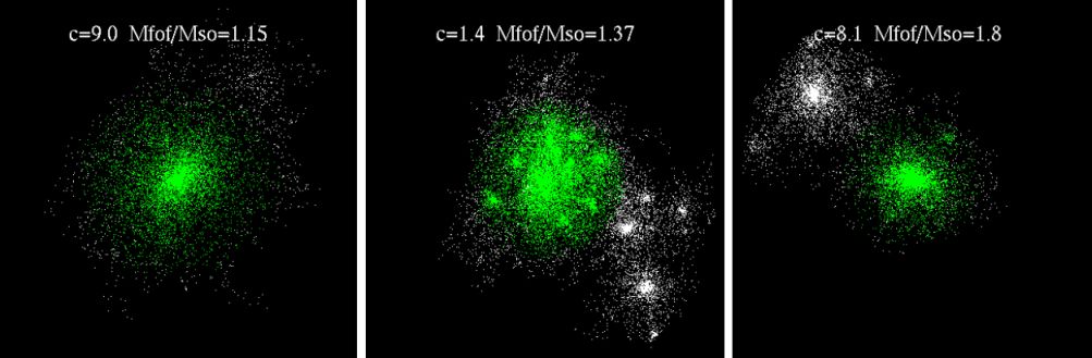Figure 3. Three examples of halos identified under both FOF (white and green colored particles) and SO (green only) algorithms. The mass ratio for each case is given, as is the concentration parameter, c, derived from a radial density fit. See text for details. Adapted from Lukić et al., (2009).

The discrepant cases do not dominate in number, but neither are they uncommon. For cosmological studies, what is important is to establish an accurate accounting process to enumerate observable halo features. Roughly speaking, observers viewing the systems in Figure 3 would be likely to identify one dominant cluster in the left and middle panels, and two in the right. An FOF accounting system would need to admit a non-unitary condition (one halo maps to two clusters) when converting mass to observable signals. In contrast, SO masses map to integrated aperture observations more directly. For this reason, SO masses see more frequent use for survey data analysis.

2.3.2. HALO MASS FUNCTION AND CLUSTERING

The original multiplicity function paper of Press & Schechter (1974) used the clustering of particles in N-body experiments with N = 1000 to support their analytic form for f(σ) in Equation 3. Later, Sheth & Tormen (1999) used N = 10⁷ simulations to set free parameters of their f(σ) model derived using an ellipsoidal, rather than spherical, collapse approximation. Using a suite of simulations of open and flat cosmologies with Ω_m ranging from 0.3 to 1, Jenkins et al. (2001) found a unique, three-parameter form for f(σ) that produced a mass function accurate to ∼ 30% across the suite of models.

A recent study by Tinker et al. (2008) employs 22 large (N ∼ 10⁹) simulations produced with three independent N-body codes to calibrate a functional form motivated by Sheth & Tormen (1999),

(13)

This study was the first to open the density threshold degree of freedom; their fitting parameters are published as functions of Δ (against _m(z)) for Δ ∈ [200, 3200]. With the high statistical power of their simulation ensemble, Tinker et al. (2008) achieve a fit with 5% statistical precision in halo number at z = 0 for a ΛCDM cosmology. Maintaining this precision for redshifts z ≤ 2.5 requires the introduction of mild redshift dependence into the fit parameters, A(z), a(z) and b(z). The theoretically expected halo counts above masses M₂₀₀ = 10¹⁴ and 10¹⁵ M_⊙ in the reference ΛCDM cosmology, shown in Figure 1, are based on the Tinker form for threshold Δ = 200 against the mean mass density (see fitting formulae in Mortonson, Hu & Huterer 2011).

On the other hand, the bias function measured in the same simulation ensemble shows no need for such redshift-dependent corrections. Framed in terms of the normalized linear perturbation amplitude, ν ∝ σ(M)⁻¹, Tinker et al. (2010) find a robust fit of the form

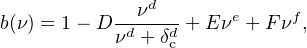(14)

with a single set of parameters {d, e, f, D, E, F} that are written only as functions of Δ. For the case ν = 3 (i.e., 3 σ peaks), the value of the bias is large, b ∼ 6, for Δ = 200. The cluster power spectrum, Equation 4, can be enhanced by factors of several tens over the mass power spectrum.

The very massive end of the FOF mass function was recently revised by Crocce et al. (2010) using 2048³-particle simulations in ΛCDM cubic volumes up to 7680 h⁻¹ in scale. Above 10¹⁵ h⁻¹ M_⊙, their fit lies up to 30% above prior calibrations (Jenkins et al. 2001; Warren et al. 2006).

2.3.3. INTERNAL HALO STRUCTURE

Gravitational relaxation drives the phase-space structure of halos to a common structure that applies from small galactic satellites to the most massive galaxy clusters. The form of the radial density,

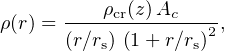(15)

is known as the Navarro-Frenk-White (NFW) profile (Navarro, Frenk & White 1995). Here, r_s is the scale radius, c is the concentration parameter (with c = r₂₀₀ / r_s) and A_c = 200 c³ / 3 [ ln(1 + c) − c / (1 + c)].

Simulations show that concentration and mass are weakly correlated. In the mass range of galaxies to clusters, c ∝ M^−ζ, with ζ ∼ 0.14 at z = 0 and ζ → 0 at z ≳ 3 (e.g., Gao et al. 2008). That study finds that a fixed concentration, c ∼ 4 ± 1, applies in the mean to high mass halos, independent of redshift. Tracking the mass accretion histories of halos in simulations, Wechsler et al. (2002) find a common functional form, and show that the formation epoch correlates strongly with concentration. The concentration–mass relation can be understood as a result of adiabatic contraction of differently-shaped peaks in the linear density field (Dalal, Lithwick & Kuhlen 2010).

2.4. From Halos to Clusters: Mass Proxies, Scaling Relations and Projection Effects

Cluster cosmology originates from phenomena observed on the sky, in the 2+1 space of angular coordinates and redshift. The observables employed for a likelihood analysis must be predicted under a set of combined cosmological and astrophysical parameters, {θ, α}. For constraints based on cluster counts, the mass function, n(M, z), written in terms of spherical overdensity or percolation measures from simulations needs to be translated into a signal function, n(S, z), for one or more signals, S_i. We use the terms signal and observable interchangeably, and generically they refer to bulk measures at mm (SZ decrement Y), optical (richness, N_gal, or velocity dispersion, σ_gal), or X-ray (luminosity, L_X; temperature, T_X; gas mass, M_gas; and/or gas thermal energy, Y_X = kT_X M_gas) wavelengths (see Section 3). An ideal experiment would measure all of these observables within apertures optimally matched to the underlying halo sizes, r_Δ(M, z). This ideal is often frustrated by signal-to-noise constraints and confused by projection effects and foreground/background contamination.

2.4.1. OBSERVABLE SIGNAL LIKELIHOOD FROM MULTIVARIATE SCALING RELATIONS

Scaling relations for cluster signals, based on assumptions of virial equilibrium and self-similar internal structure, were first published by Kaiser (1986). In this model, halos at fixed mass and redshift are identical, and scalings with mass and redshift follow calculated power-law behaviors. Observations generally support power-law behavior, but not always with the self-similar slope (Section 4.1.3). We describe here a non-self-similar model that incorporates arbitrary mass scaling and allows for variations at fixed mass and redshift.

For compactness of notation, let s_i = ln(S_i), for each of the N observables, S_i, and let µ = lnM. The power-law assumption transforms to log-linear scaling

(16)

where the average is over a very large cosmic volume. The elements of m are the slopes of the individual mass-observable relations, and the intercepts b(z) reflect the evolution at fixed mass. At a fixed epoch, we can always choose units such that b_i(z) = 0 (as we do below). For cosmological studies, a measure of merit is the equivalent mass scatter in each signal, σ_{µ i} ≡ σ_i / m_i.

Various processes, including different formation histories and the stochastic nature of mergers, generate deviations from the mean. Taking these as Gaussian in the log leads to a form for the conditional signal likelihood,

(17)

The elements of the covariance matrix, Ψ_ij ≡ ⟨(s_i − s_i) (s_j − s_j) ⟩, could have mass or redshift dependence, but a first-order approach considers them as constants.

When the mass variance of signals is small, σ_{µ i}² ≪ 1, then the above expressions can be convolved with a locally power-law approximation to the mass function, n(µ, z) = A e^{−a µ}, to obtain the local signal space density function,

(18)

where Σ² = ( m^† Ψ⁻¹ m )⁻¹ is the variance about the mean log-mass selected by the set of signals s,

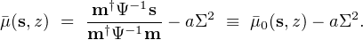(19)

The first term above is the mean mass for the case of a flat mass function, a = 0. The second term, represents the (Eddington) mass bias induced by asymmetry in the mass function convolution. Upscattering of low-mass systems dominates when a > 0, and the high-mass end of the ΛCDM mass function is steep, a ≳ 3 (Mortonson, Hu & Huterer 2011). These equations make explicit the degeneracy between cosmology (e.g. A and a) and astrophysics (e.g. m and Ψ) inherent in cluster counts. They provide the means to compute biases, relative to a mass complete sample, associated with signal-limited cluster samples (discussed further in Section 2.5.1).

Figure 4 provides support for this model from Millennium Gas Simulation analysis (Stanek et al. 2010). The left panel shows deviations about the mean behavior of four intrinsic (3-dimensional) properties measured within r₂₀₀ for > 4500 halos with mass M₂₀₀ > 5 × 10¹³ h⁻¹ M_⊙ at z = 0. The lower diagonal and red histograms show results from a cooling and preheating (PH) treatment of the baryons, where the entropy is instantaneously raised to 200 keV cm² at z = 4. Only a small fraction of baryons cool into stars in this model (Young et al. 2011). The upper diagonal and blue histograms are from a gravity-only (GO) treatment, where the gas is heated only by shocks and does not cool.

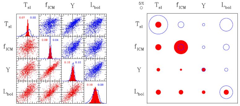Figure 4. Left: Covariance of internal properties of > 4500 halos with M200 > 5 × 1013 h−1 M⊙ extracted from Millennium Gas Simulations produced under two different physical treatments. Off-diagonal panels show normalized ((si − si) / σi) pairwise deviations under preheating (PH, lower) and gravity-only (GO, upper) treatments; large tickmarks are separated by unity. Diagonal panels show the distribution of ln(property) deviations for PH (red) and GO (blue) models, with dispersions given in the legend. Right: Visual representation of the mass variance, Equation 20, obtained using the property pairs at left. The radii scale with Σ, and a 5% reference is shown in the upper left. Adapted from Stanek et al. 2010.

The internal properties generally have modest variance, and pairs tend to be positively correlated with typical correlation coefficient r ∼ 0.4−0.8. Halos identified by a pair of properties will have mass variance

(20)

shown by the areas of the off-diagonal circles in the right panel of Figure 4. Individual properties lie along the diagonal. The intrinsic gas thermal energy, Y, selects mass with 7% dispersion, the best individual measure for both physics cases. This level is also seen in the simulations of Nagai (2006) which include cooling, star formation and feedback. Pairs of intrinsic measurements always improve mass selection, and the strong correlation between f_ICM and Y combines with the large mass variance of f_ICM to achieve mass selection with 4% scatter in the PH model.

Applying Bayes’ theorem to this model allows one to write the likelihood of mass and an observable, s₂, for a sample selected on observable s₁. When the two signals are correlated, one can show that the scaling with mass of the non-selection signal will be

(21)

which is biased relative to the naive expectation of m₂ s₁ / m₁. The intrinsic correlation between signals at fixed mass is relatively challenging to constrain from current data, but first measurements have been made for samples selected using optical (Rozo et al. 2009) and X-ray (Mantz et al. 2010a) observations.

2.5. From Theory to Practice: Sources of Systematic Error

Clusters on the sky relate to halos through selection on one or more observables. Matching cluster detections (which originally reside in a 2+1 space of angular position and signal-to-noise) to halos can sometimes be complex; two halos along nearly the same line of sight may be blended into a single cluster, or a single halo may be fragmented into more than one cluster. The frequency of these occurrences is typically not large, ≲ 10%, but the exact values are sensitive to a number of factors, particularly detection method and mass, and so are best modeled via direct sky realizations (e.g. Sehgal et al. 2011).

The selection observable can be distorted from its intrinsic value (Equation 17) by triaxiality, by additional sources along the line-of-sight, by mis-centering and/or mis-estimation of the radial scale, and by other effects. Telescope/instrument calibration and data processing methods also contribute to the error budget. For upcoming studies using cluster counts, photometric redshift errors have an important, but not dominant, effect (Section 6.1).

2.5.1. SAMPLE SELECTION

Testing cosmology with halo counts and clustering requires that the theoretical mass function be transformed, via the scaling relations and a model of the selection process, into a prediction for the distribution of clusters in the space of survey observables (e.g. redshift and X-ray flux). The scaling relation parameters set the space density portion of the survey yield (Equation 18) in terms of the (cosmologically dependent) local amplitude, A(µ, z), and logarithmic slope, a(µ, z), of the mass function. Sample selection must be well understood to avoid perturbing A(µ, z) and a(µ, z) from their true values, biasing cosmological results. Fortunately, such effects can be mitigated by survey self-calibration (Majumdar & Mohr 2004) or by calibration using follow-up observations, as discussed below.

The task of empirically constraining the scaling relations is complicated by the fact that the clusters targeted for follow-up observations are themselves subject to selection effects related to their original discovery. In an X-ray flux-limited sample, for example, higher X-ray luminosity at a given mass leads to a larger probability of detection (commonly known as Malmquist bias). The effects of selection bias must therefore be accounted for in the calibration of scaling relations, much as in the cosmological analysis (e.g. Stanek et al. 2006; Sahlén et al. 2009).

Figure 5 illustrates the influence of selection on observed scaling relation data in a cartoon case. The full population (black crosses and green points) obeys a scaling law (red line) with non-trivial intrinsic scatter. In the simple case where detection requires a particular threshold luminosity (the dashed, blue line), it can be seen that, even if every detected cluster is followed up to obtain precise measurements of the mass and luminosity, the resulting data set will be a biased representation of the full population. While complete at the highest masses, the sample is increasingly incomplete at low masses, with the low-luminosity systems absent.

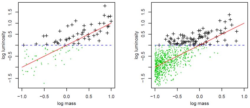Figure 5. Cartoon illustrating generically how the distribution of observed scaling relation data (black crosses) do not reflect the underlying scaling law (red line) due to selection effects (e.g. a luminosity threshold; blue, dashed line). Green dots indicate undetected sources. The left panel shows an unphysical case in which cluster log-masses are uniformly distributed, while the mass function in the right panel is a more realistic, steeper power-law (normalized to produce roughly the same number at high masses). The steepness of the mass function has a clear effect on the degree of bias in the detected sample. To recover the correct scaling relation, an analysis must account for both the selection function of the data and the underlying mass function of the cluster population. Adapted from Mantz et al. (2010a).

A closely related consideration is the effect of the underlying mass function on the observed scaling relation data. The distribution of the relation’s independent variable(s) (in this case cluster masses) within the full population generically influences constraints on scaling laws (e.g. Gelman et al. 2004; Kelly 2007). Neglecting to account for this influence corresponds to the assumption of uniformly distributed independent variables; often this approximation is sufficient, but the exponentially steep slope of the cluster mass function suggests that we should take the issue seriously in the context of cluster cosmology (Mantz et al. 2010b). Figure 5 illustrates how the steepness of the mass function influences the fraction of the observed data which are strongly biased relative to the underlying scaling relation. Given the need to solve for both the slope and scatter of the scaling relation, accounting for the disparity in the number of high-mass and low-mass systems is critical. We note that simply conditioning the sampling distribution on cluster detection, as some authors have done, is not sufficient to rigorously recover all the scaling information.

Note that this effect has a floor set by non-zero intrinsic scatter in the scaling relations, but the effect can in principle be enhanced by measurement error. However, measurement errors in current X-ray and optical cluster surveys are typically smaller than the intrinsic dispersion, even at the survey limit. Thus, re-measurement of the survey observables through deeper, follow-up observations (e.g. to improve the signal-to-noise of X-ray or SZ flux) does not circumvent the issue of selection bias in the scaling relation analysis.

While selection bias clearly influences scaling relations involving the selection observable, it also influences relations of other signals with which the selection observable has non-zero intrinsic correlation (Equation 21). This is illustrated in Figure 6, for a signal which is correlated with the selection observable with coefficient 0.1 (left panel) and 0.9 (right panel). The red line shows the true scaling law and the points shown correspond to the detected clusters from Figure 5 (right panel). With relatively mild intrinsic correlation, as has been found for temperatures and soft X-ray flux detection (Mantz et al. 2010a), the distribution of data points closely follows the underlying relation; for more extreme values of the correlation coefficient, as might be expected, e.g., between temperature and SZ signal, deviations due to selection bias become evident. Note that the severity of the effect also depends on the covariance of the signals rather than only on the correlation coefficient (i.e. the size of the marginal scatter in each signal is also important).

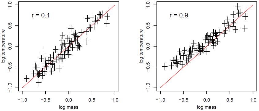Figure 6. Cartoon scaling relations where the observable of interest is not the basis of cluster selection. In both panels, the red line indicates the true scaling relation, and the black crosses correspond to the detected clusters in the right panel of Figure 5. The marginal scatter in this relation is chosen to be smaller than that in Figure 5, consistent with measured values of the luminosity–mass and temperature–mass intrinsic scatters (Section 3.3.4). The intrinsic temperature–luminosity correlation at fixed mass is relatively small in the left panel (r = 0.1) and large in the right panel (r = 0.9); in the latter case, the observed data are significantly influenced by selection bias despite the fact that the selection was made using a different observable.

Cluster samples are often characterized in terms of completeness and purity (White & Kochanek 2002). Completeness is used in many ways, but its simplest form for cluster cosmology refers to the fraction of halos above mass M at redshift z that are identified in a survey with some observable limit, S_lim(z). Completeness of unity is achievable at high masses when the survey limit, S_lim(z), lies sufficiently far in the signal likelihood’s negative tail. Impurity is a measure of false positive sources in the sample. Fewer conventions for its definition exist in the literature. Generically, one can write the observed counts above some signal limit S as a sum, N_obs(> S) = N_true(> S) + N_false(> S), where the first term represents genuine cluster systems – manifestations of a single massive halo along the line of sight – and the second expresses detections of other origin. Zero impurity, N_false(> S) = 0, is a desired goal.

2.5.2. PROJECTION EFFECTS

Telescopes aimed at a distant halo necessarily collect photons that originate elsewhere along the multi-gigaparsec sightline than within the target system. Due to their softer angular profiles, SZ, lensing and optical cluster signals can be blended more readily than X-ray. Chance orientations of two or more halos within local supercluster regions create an asymmetric tail to high signal values. Considered in terms of mass selection, the effect produces a tail to low masses in the distribution of halo mass selected at a given signal (e.g. Cohn et al. 2007).

Since the matter components of halos are generally ellipsoidal rather than spherical, orientation variations also produce scatter in signals observed in halos of fixed mass. Signals are generally maximized when viewed along the long axis and minimized along the short axis. Orientation can affect cluster selection, with prolate systems oriented along the line-of-sight being preferentially included. Since its collisional nature drives the X-ray emitting gas toward equipotential surfaces, it tends to be rounder than the dark matter and so less susceptible to orientation bias.

As discussed in Section 3, the density squared dependence of the X-ray emissivity means that X-ray selection is less prone to projected confusion. Optical richness measurements roughly trace mass density and are therefore more easily confused by projection and orientation effects. SZ measurements are intermediate, since the SZ effect depends on electron pressure, the product of density and temperature.

2.6. Non-Standard Scenarios

It is important to keep in mind that theory offers many potential deviations from the reference ΛCDM cosmology sketched above. Key model assumptions – that the dark matter is a weakly interacting massive particle, that inflation produced a Gaussian spectrum of initial density fluctuations with a power-law initial spectrum, that small-amplitude metric perturbations are well described by Newtonian, weak field expansions in general relativity, and so on – need to be rigorously tested. In Section 5, we discuss ways in which clusters can be used to test a number of proposed modifications to the reference model.