NOTES ON STATISTICS FOR PHYSICISTS, REVISED
Jay Orear
Laboratory for Nuclear Studies
Cornell University
Ithaca, NY 14853
Table of Contents
 ORIGINAL PREFACE
- PREFACE TO REVISED EDITION
- DIRECT PROBABILITY
- INVERSE PROBABILITY
- LIKELIHOOD RATIOS
- MAXIMUM-LIKELIHOOD METHOD
- GAUSSIAN DISTRIBUTIONS
- MAXIMUM-LIKELIHOOD ERROR, ONE PARAMETER
- MAXIMUM-LIKELIHOOD ERRORS, M-PARAMETERS CORRELATED
ERRORS
- PROPAGATION OF ERRORS: THE ERROR MATRIX
- SYSTEMATIC ERRORS
- UNIQUENESS OF MAXIMUM-LIKELIHOOD SOLUTION
- CONFIDENCE INTERVALS AND THEIR ARBITRARINESS
- BINOMIAL DISTRIBUTION
- POISSON DISTRIBUTION
- GENERALIZED MAXIMUM-LIKELIHOOD METHOD
- THE LEAST-SQUARES METHOD
- GOODNESS OF FIT, THE
 2
DISTRIBUTION
2
DISTRIBUTION
- APPENDIX I: PREDICTION OF LIKELIHOOD RATIOS
- APPENDIX II: DISTRIBUTION OF THE LEAST-SQUARES SUM
- APPENDIX III. LEAST SQUARES WITH ERRORS IN BOTH
VARIABLES
- APPENDIX IV. NUMERICAL METHODS FOR MAXIMUM
LIKELIHOOD AND LEAST SQUARES SOLUTIONS
- APPENDIX V. CUMULATIVE GAUSSIAN AND CGI-SQUARED
DISTRIBUTIONS
- REFERENCES
ORIGINAL PREFACE
These notes are based on a series of lectures given at
the Radiation Laboratory in the summer of 1958. I wish to
make clear my lack of familiarity with the mathematical literature
and the corresponding lack of mathematical rigor in this
presentation. The primary source for the basic material and
approach presented here was Enrico Fermi. My first introduction
to much of the material here was in a series of discussions with
Enrico Fermi, Frank Solmitz, and George Backus at the University
of Chicago in the autumn of 1953. I am grateful to Dr. Frank
Solmitz for many helpful discussions and I have drawn heavily
from his report "Notes on the Least Squares and Maximum Likelihood
Methods." [1]
The general presentation will be to study the
Gausssian distribution, binomial distribution, Poisson distribution,
and least-squares method in that order as applications
of the maximum-likelihood method.
August 13, 1958
PREFACE TO REVISED EDITION
Lawrence Radiation Laboratory has granted permission to
reproduce the original UCRL-8417. This revised version
consists of the original version with corrections and clarifications
including some new topics. Three completely new appendices have
been added.
Jay Orear
July 1982
1. DIRECT PROBABILITY
Books have been written on the "definition" of probability.
We shall merely note two properties: (a) statistical
independence (events must be completely unrelated), and
(b) the law of large numbers. This says that if
p1 is the
probability of getting an event in Class 1 and we observe
that N1 out of N events are in Class 1, then we
have
A common example of direct probability in physics is that in
which one has exact knowledge of a final-state wave function
(or probability density). One such case is that in which we
know in advance the angular distribution f (x), where
x = cos of a certain scattering experiment, In this example one can
predict with certainty that the number of particles that
leave at an angle x1 in an interval
of a certain scattering experiment, In this example one can
predict with certainty that the number of particles that
leave at an angle x1 in an interval
 x1 is
Nf
(x1)x1,
where N, the total number of scattered particles, is a very large
number. Note that the function f(x) is normalized to unity:
x1 is
Nf
(x1)x1,
where N, the total number of scattered particles, is a very large
number. Note that the function f(x) is normalized to unity:
As physicists, we call such a function a distribution function.
Mathematicians call it a probability density function. Note
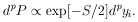
that an element of probability, dp, is
2. INVERSE PROBABILITY
The more common problem facing a physicist is that he
wishes to determine the final-state wave function from
experimental measurements. For example, consider the decay of a
spin-½ particle, the muon, which does not conserve parity.
Because of angular-momentum conservation, we have the a priori
knowledge that
However, the numerical value of
 is some universal physical
constant yet to be determined. We shall always use the
subscript zero to denote the true physical value of the parameter
under question. It is the job of the physicist to determine
0. Usually the
physicist does an experiment and
quotes a result =
* ±
. The major
portion of this report is devoted to the questions, What do we mean by
* and
? and What is the "best" way to
calculate * and
? These
are questions of extreme importance to all physicists.
is some universal physical
constant yet to be determined. We shall always use the
subscript zero to denote the true physical value of the parameter
under question. It is the job of the physicist to determine
0. Usually the
physicist does an experiment and
quotes a result =
* ±
. The major
portion of this report is devoted to the questions, What do we mean by
* and
? and What is the "best" way to
calculate * and
? These
are questions of extreme importance to all physicists.
Crudely speaking,
is the standard deviation,
[2] and what
the physicist usually means is that the "probability" of finding
(the area under a Gaussian curve out to one standard deviation).
The use of the word "probability" in the previous sentence would
shock a mathematician. He would say the probability of having
The kind of probability the physicist is talking about here we
shall call inverse probability, in contrast to the direct
probability used by the mathematician. Most physicists use the
same word, probability, for the two completely different
concepts: direct probability and inverse probability. In the
remainder of this report we will conform to this sloppy
physicist-usage of the word "probability."
3. LIKELIHOOD RATIOS
Suppose it is known that either Hypothesis A or Hypothesis
B must be true. And it is also known that if A is true the
experimental distribution of the variable x must be
fA(x), and
if B is true the distribution is fB(x). For
example, if
Hypothesis A is that the K meson has spin zero, and hypothesis
B that it has spin 1, then it is "known" that
fA(x) = 1 and
fB(x) = 2x, where x is the kinetic
energy of the decay  -
divided by its maximum value for the decay mode
K+ ->
- +
2+.
-
divided by its maximum value for the decay mode
K+ ->
- +
2+.
If A is true, then the joint probability for getting a
particular result of N events of values
x1, x2,..., xN is
The likelihood ratio is

| (1)
|
This is the probability, that the particular experimental result
of N events turns out the way it did, assuming A is true, divided
by the probability that the experiment turns out the way it did,
assuming B is true. The foregoing lengthy sentence is a correct
statement using direct probability. Physicists have a shorter
way of saying it by using inverse probability. They say
Eq. (1) is the betting odds of A against B. The formalism of
inverse probability assigns inverse probabilities whose ratio
is the likelihood ratio in the case in which there exist
no prior probabilities favoring A or B.
[3] All the remaining
material in this report is based on this basic principle alone.
The modifications applied when prior knowledge exists are
discussed in Sec. 10.
An important job of a physicist planning new experiments
is to estimate beforehand how many events he will need to
"prove" a hypothesis. Suppose that for the K+ ->
- +
2+ one
wishes to establish betting odds of 104 to 1 against spin 1.
How many events will be needed for this? The problem and the
general procedure involved are discussed in
Appendix I: Prediction of Likelihood Ratios.
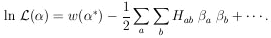
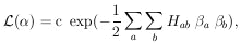
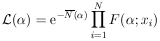
4. MAXIMUM-LIKELIHOOD METHOD
The preceding section was devoted to the case in which one
had a discrete set of hypotheses among which to choose. It is
more common in physics to have an infinite set of hypotheses;
i.e., a parameter that is a continuous variable. For example,
in the µ-e decay distribution
the possible values for
0 belong to a
continuous rather than a
discrete set. In this case, as before, we invoke the same basic
principle which says the relative probability of any two different
values of is the ratio of
the probabilities of getting our
particular experimental results, xi, assuming first
one and then
the other, value of is
true. This probability function of
is called the likelihood function,
 ().
().
The relative probabilities of
can be displayed as a plot of
() vs.
. The most probable value of
is
called the maximum-likelihood solution
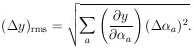
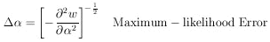
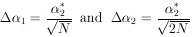
*. The rms (root-mean-square)
spread of about
* is a conventional measure
of the accuracy of the
determination =
* . We shall call this
.
| (3)
|
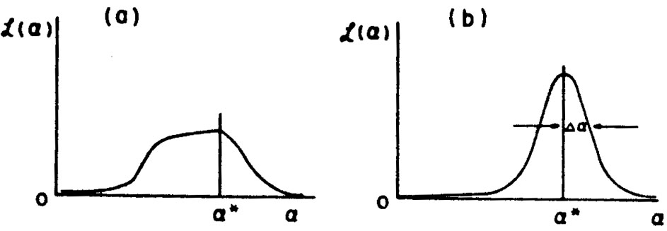
In general, the likelihood function will be close to Gaussian
(it can be shown to approach a Gaussian distribution as
N ->  )
and will look similar to Fig. 1b.
)
and will look similar to Fig. 1b.
Fig. 1a represents what is called a case of poor
statistics. In
such a case, it is better to present a plot of
() rather than merely quoting
* and
. Straightforward
procedures for obtaining
are presented in
Sections 6 and 7.
A confirmation of this inverse probability approach is the
Maximum-Likelihood Theorem, which is proved in Cramer
[4] by use
of direct probability. The theorem states that in the limit of
large N,
* ->
0; and
furthermore, there is
no other method of estimation that is more accurate.
In the general case in which there are M parameters,
1, ...,
M, to be
determined, the procedure for obtaining the
maximum likelihood solution is to solve the M simultaneous
equations,
| (4)
|
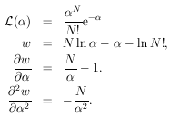
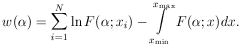
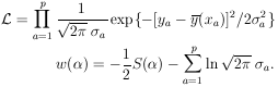
5. GAUSSIAN DISTRIBUTIONS
As a first application of the maximum-likelihood method,
we consider the example of the measurement of a physical
parameter 0,
where x is the result of a particular type of
measurement that is known to have a measuring error
 . Then
if x is Gaussian-distributed, the distribution function is
. Then
if x is Gaussian-distributed, the distribution function is
For a set of N measurements xi, each with its
own measurement
error i the
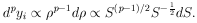
likelihood function is
then

| (5)
|
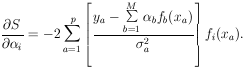
The maximum-likelihood solution is

| (6)
|
Note that the measurements must be weighted according to the
inverse squares of their errors. When all the measuring errors
are the same we have
Next we consider the accuracy of this determination.
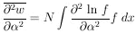
6. MAXIMUM-LIKELIHOOD ERROR, ONE PARAMETER
It can be shown that for large N,
() approaches a
Gaussian distribution. To this approximation (actually the
above example is always Gaussian in
), we have
where
1 /  h is the rms spread
of about
*,
h is the rms spread
of about
*,
Since as defined in Eq. (3) is
1 / h , we have
| (7)
|
It is also proven in Cramer
[4] that no method of
estimation
can give an error smaller than that of Eq. 7 (or its alternate
form Eq. 8). Eq. 7 is indeed very powerful and important. It
should be at the fingertips of all physicists. Let us now
apply this formula to determine the error associated with
* in
Eq. 6. We differentiate Eq. 5 with respect to
. The answer is
Using this in Eq. 7 gives
This formula is commonly known as the law of combination of
errors and refers to repeated measurements of the same quantity
which are Gaussian-distributed with "errors"
i.
In many actual problems, neither
* nor
may be found
analytically. In such cases the curve
() can be
found numerically by trying several values of
and using Eq. (2) to
get the corresponding values of
(). The complete function
is then obtained by drawing a smooth curve through the points. If
() is Gaussian-like,
ð2w /
ð2
is the same everywhere. If not, it is best to use the average
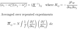
A plausibility argument for using the above average goes as
follows: If the tails of
() drop off more slowly than
Gaussian tails,
 is smaller than
Thus, use of the average second derivative gives the required
larger error.
Note that use of Eq. 7 for
depends on having a particular
experimental result before the error can be determined.
However, it is often important in the design of experiments to
be able to estimate in advance how many data will be needed in
order to obtain a given accuracy. We shall now develop an
alternate formula for the maximum-likelihood error, which
depends only on knowledge of
f (; x). Under
these circumstances we wish to determine
averaged over many repeated experiments
consisting of N events each. For one event we have
for N events
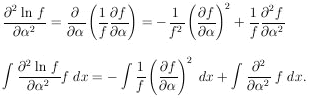
This can be put in the form of a first derivative as follows:
The last integral vanishes if one integrates before the
differentiation because
Thus
and Eq. (7) leads to
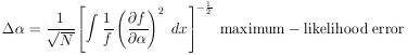
| (8)
|
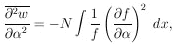
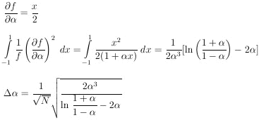
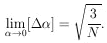
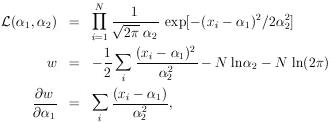
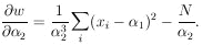
Example 1
Assume in the µ-e decay distribution function,
f (; x) =
(1 + x) / 2 ,
that
0 = - 1/3. How
many µ-e decays are needed to establish a
to a 1% accuracy (i.e.,
/
= 100)?
Note that
For
For this problem
7. MAXIMUM-LIKELIHOOD ERRORS, M-PARAMETERS CORRELATED ERRORS
When M parameters are to be determined from a single experiment
containing N events, the error formulas of the preceding
section are applicable only in the rare case in which the errors
are uncorrelated.. Errors are uncorrelated only for
 = 0 for all
cases with
i
= 0 for all
cases with
i  j. For the
general case we Taylor-expand
w() about
(*):
j. For the
general case we Taylor-expand
w() about
(*):
where
and
| (9)
|
The second term of the expansion vanishes because
ðw / ð = 0
are the equations for *
Neglecting the higher-order terms, we have
(an M-dimensional Gaussian surface). As before, our error
formulas depend on the approximation that
() is
Gaussian-like in the region
i
 i*. As mentioned in
Section 4, if the
statistics are so poor that this is a poor approximation, then
one should merely present a plot of
(). (see Appendix IV).
i*. As mentioned in
Section 4, if the
statistics are so poor that this is a poor approximation, then
one should merely present a plot of
(). (see Appendix IV).
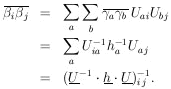
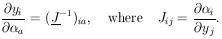
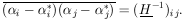
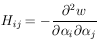
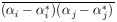
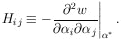
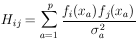
According to Eq. (9), H is a symmetric matrix. Let
U
be the unitary matrix that diagonalizes H:
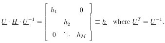
| (10)
|
Let
 and
and
 . The
element of
probability in the
. The
element of
probability in the  -space is
Since
|U| = 1 is the Jacobian relating the volume elements
dM and
dM , we have
Now that the general M-dimensional Gaussian surface has been
put in the form of the product of independent one-dimensional
Gaussians we have
Then
According to Eq. (10),
H = U-1
. h . U, so that the final
result is
| Maximum
Likelihood
Errors,
M parameters (11)
|
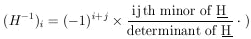
(A rule for calculating the inverse matrix
H-1 is
If we use the alternate notation
V for the error matrix
H-1, then whenever
H appears, it must be replaced with
V-1; i.e.,
the likelihood function is
| (11a)
|
Example 2
Assume that the ranges of monoenergetic particles are
Gaussian-distributed with mean range
1 and straggling
coefficient
2 (the standard
deviation). N particles having ranges
x1,..., xN are observed. Find
1*,
2*, and their
errors . Then
The maximum-likelihood solution is obtained by setting the
above two equations equal to zero.
The reader may remember a standard-deviation formula in which N
is replaced by (N - 1):
This is because in this case the most probable value,
2*, and
the mean,
 2 ,
do not occur at the same place. Mean
values of
such quantities are studied in Section 16.
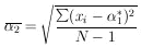
The matrix H is
obtained by evaluating the following quantities at
1* and
2*:
2 ,
do not occur at the same place. Mean
values of
such quantities are studied in Section 16.
The matrix H is
obtained by evaluating the following quantities at
1* and
2*:
According to Eq. (11), the errors on
1 and
2 are the
square
roots of the diagonal elements of the error matrix, H-1:
| (this is sometimes
called the
error of the error).
|
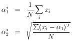
We note that the error of the mean is
1/sqrt[N]
where
=
2 is
the standard deviation. The error on the determination of
is
/sqrt[2N].
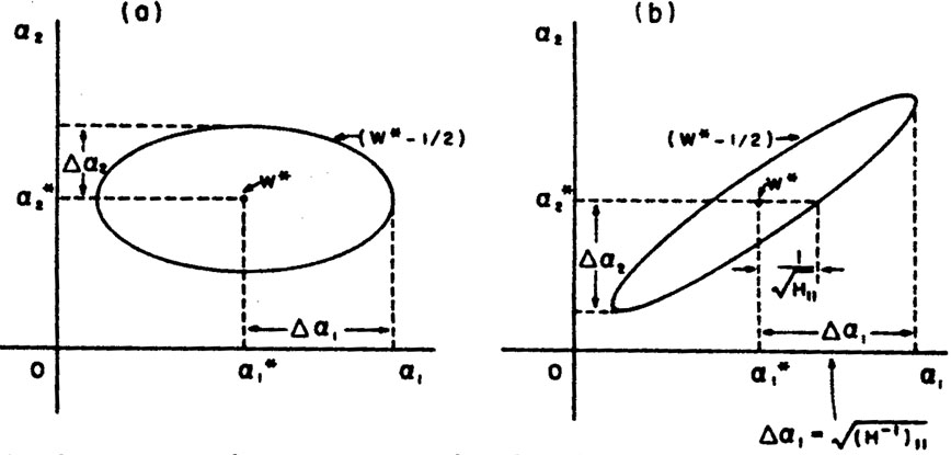
Correlated Errors
The matrix
Vij  is
defined as the error matrix (also called the covariance matrix of
). In Eq. 11
we have shown that
V = H-1 where
Hij = - ð2 w /
(ði
ðj). The
diagonal elements of V are the variances of the
's. If all the
off-diagonal elements are zero, the errors in
are uncorrelated
as in Example 2. In this case contours of constant w plotted
in (1,
2) space would be
ellipses as shown in Fig. 2a. The
errors in 1 and
2 would be the
semi-major axes of the contour ellipse where w has dropped by
½ unit from its maximum-likelihood
value. Only in the case of uncorrelated errors is the rms error
j =
(Hjj)-½ and then there is no
need to perform a matrix inversion.
is
defined as the error matrix (also called the covariance matrix of
). In Eq. 11
we have shown that
V = H-1 where
Hij = - ð2 w /
(ði
ðj). The
diagonal elements of V are the variances of the
's. If all the
off-diagonal elements are zero, the errors in
are uncorrelated
as in Example 2. In this case contours of constant w plotted
in (1,
2) space would be
ellipses as shown in Fig. 2a. The
errors in 1 and
2 would be the
semi-major axes of the contour ellipse where w has dropped by
½ unit from its maximum-likelihood
value. Only in the case of uncorrelated errors is the rms error
j =
(Hjj)-½ and then there is no
need to perform a matrix inversion.
In the more common situation there will be one or more
off-diagonal elements to
H and the errors are correlated
(V has
off-diagonal elements). In this case (Fig. 2b)
the contour ellipses are inclined to the
1,
2 axes. The rms
spread of 1
is still 1 =
sqrt[V11], but it is the extreme limit of
the ellipse projected on the
1-axis. (The
ellipse "halfwidth" axis is
(H11)-½ which is smaller.) In cases
where Eq. 11 cannot be evaluated analytically, the
*'s can be found numerically and
the errors in can be found
by Plotting the ellipsoid where
w is 1/2 unit less than w * . The
extremums of this ellipsoid are
the rms error in the 's. One
should allow all the
j to change
freely and search for the maximum change in
i which makes
w = (w * - ½). This maximum
change in
i, is the
error in i and is
sqrt[V11].
8. PROPAGATION OF ERRORS: THE ERROR MATRIX
Consider the case in which a single physical quantity, y,
is some function of the 's:
y = y(1, ...,
M). The "best"
value for y is then y* =
y(i*).
For example y could be the path
radius of an electron circling in a uniform magnetic field where
the measured quantities are
1 =
 , the period of revolution,
and
2 = v, the
electron velocity. Our goal is to find the
error in y given the errors in
. To first order in
(i -
i*) we have
, the period of revolution,
and
2 = v, the
electron velocity. Our goal is to find the
error in y given the errors in
. To first order in
(i -
i*) we have
| (12)
|
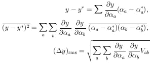
A well-known special case of Eq. (12), which holds only when
the variables are completely uncorrelated, is
In the example of orbit radius in terms of
and v this becomes
in the case of uncorrelated errors. However, if
 is
non-zero as one might expect, then Eq. (12) gives
is
non-zero as one might expect, then Eq. (12) gives
It is a common problem to be interested in M physical parameters,
y1, ..., yM, which are known
functions of the
i.
In fact the yi can be thought of as a new set of
i or a
change of basis from
i to
yi. If the error matrix of the
i
is known, then we have

| (13)
|
In some such cases the ðyi /
ða cannot be
obtained directly, but the
ði /
ðya are easily
obtainable. Then
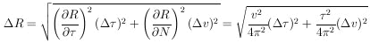
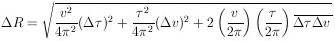
Example 3
Suppose one wishes to use radius and acceleration to
specify the circular orbit of an electron in a uniform magnetic
field; i.e., y1 = r and y2 =
a. Suppose the original measured quantities are
1 =
= (10 ± 1)µs and
2 = v =
(100 ± 2) km/s. Also
since the velocity measurement depended on the time measurement,
there was a correlated error
= 1.5 × 10⁻³
m. Find
r,r, a,
a.
Since r = v /
2 = 0.159 m and
a = 2v /
= 6.28 × 10¹⁰
m/s2 we have y1 =
12 /
2 and
y2 = 2
2 /
1. Then
ðy1 /
ð1 =
2 /
2,
ðy1 /
ð2 =
1 /
2,
ðy2 /
ð1 =
-22 /
12,
ðy2 /
ð2 =
2 /
1 . The
measurement errors specify the error matrix as
Eq. 13 gives
Thus r = (0.159 ± 0.184) m
For y2, Eq. 13 gives
Thus
a = (6.28 ± 0.54) × 1010 m/s2.
9. SYSTEMATIC ERRORS
"Systematic effects" is a general category which includes
effects such as background, selection bias, scanning efficiency,
energy resolution, angle resolution, variation of counter
efficiency with beam position and energy, dead time, etc. The
uncertainty in the estimation of such a systematic effect is
called a "systematic error". Often such systematic effects and
their errors are estimated by separate experiments designed for
that specific purpose. In general, the maximum-likelihood
method can be used in such an experiment to determine the
systematic effect and its error. Then the systematic effect
and its error are folded into the distribution function of
the main experiment. Ideally, the two experiments can be
treated as one joint experiment with an added parameter
M+1
to account for the systematic effect.
In some cases a systematic effect cannot be estimated
apart from the main experiment. Example 2 can be made into
such a case. Let us assume that among the beam of mono-energetic
particles there is an unknown background of particles
uniformly distributed in range. In this case the distribution
function would be
where
The solution
3* is simply
related to the percentage of background.
The systematic error is obtained using Eq. 11.
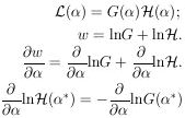
10. UNIQUENESS OF MAXIMUM-LIKELIHOOD SOLUTION
Usually it is a matter of taste what physical quantity is
chosen as . For example, in
a lifetime experiment some workers would solve for the lifetime,
*, while others would solve for
 *, where
=
1/. Some workers prefer to use
momentum, and
others energy, etc. Consider the case of two related physical
parameters and
. The maximum-likelihood
solution for is
obtained from the equation
ðw / ð = 0. The
maximum-likelihood
solution for is obtained
from
ðw / ð =
0. But then we have
*, where
=
1/. Some workers prefer to use
momentum, and
others energy, etc. Consider the case of two related physical
parameters and
. The maximum-likelihood
solution for is
obtained from the equation
ðw / ð = 0. The
maximum-likelihood
solution for is obtained
from
ðw / ð =
0. But then we have
Thus the condition for the maximum-likelihood solution is
unique and independent of the arbitrariness involved in choice
of physical parameter. A lifetime result
* would be related
to the solution
* by
* =
1/*.
The basic shortcoming of the maximum-likelihood method is
what to do about the prior probability of
. If the prior
probability of is
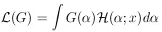
G() and the
likelihood function obtained for the experiment alone is
 (), then the joint likelihood
function is
(), then the joint likelihood
function is
give the maximum-likelihood solution. In the absence of any
prior knowledge the term on the right-hand side is zero. In
other words, the standard procedure in the absence of any prior
information is to use a prior distribution in which all values
of are equally
probable. Strictly speaking, it is impossible
to know a "true" G(),
because it in turn must depend on its
own prior probability. However, the above equation is useful
when G() is the
combined likelihood function of all previous experiments and
() is the likelihood function of
the experiment under consideration.
There is a class of problems in which one wishes to determine
an unknown distribution in
,
G(), rather than a single
value . For example, one may
wish to determine the momentum
distribution of cosmic ray muons. Here one observes
where (; x) is known from the
nature of the experiment and
G() is the function to be
determined. This type of problem is discussed in Reference 5.
11. CONFIDENCE INTERVALS AND THEIR ARBITRARINESS
So far we have worked only in terms of relative probabilities
and rms values to give an idea of the accuracy of the
determination
=
*. One can also ask the
question, What is
the probability that lies
between two certain values such as
' and
"? This is called a
confidence interval,
Unfortunately such a probability depends on the arbitrary choice
of what quantity is chosen for
. To show this consider the
area under the tail of
().
If =
() had been chosen as the physical
parameter instead, the same confidence interval is
Thus, in general, the numerical value of a confidence interval
depends on the choice of the physical parameter. This is also
true to some extent in evaluating
. Only the maximum likelihood
solution and the relative probabilities are unaffected by
the choice of . For Gaussian
distributions, confidence
intervals can be evaluated by using tables of the probability integral.
Tables of cumulative binomial distributions and cumulative
Poisson distributions are also available.
Appendix V contains
a plot of the cumulative Gaussian distribution.
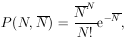
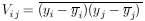
12. BINOMIAL DISTRIBUTION
Here we are concerned with the case in which an event must
be one of two classes, such as up or down, forward or back,
positive or negative, etc. Let p be the probability for an
event of Class 1. Then (1 - p) is the probability for Class 2,
and the joint probability for observing N1 events in
Class 1 out of N total events is

| The binomial
distribution
| (14)
|
Note that
 j=1N
p(j, N) = [p + (1 - p)]N =
1. The factorials correct
for the fact that we are not interested in the order in which
the events occurred. For a given experimental result of
N1 out of N events in Class 1, the likelihood
function
(p) is then
j=1N
p(j, N) = [p + (1 - p)]N =
1. The factorials correct
for the fact that we are not interested in the order in which
the events occurred. For a given experimental result of
N1 out of N events in Class 1, the likelihood
function
(p) is then

| (15)
|

| (16)
|
From Eq. (15) we have

| (17)
|
From (16) and (17):

| (18)
|
The results, Eqs. (17) and (18), also happen to be the same as
those using direct probability. Then
and
Example 4
In Example 1 on the µ-e decay angular distribution we found
that
is the error on the asymmetry parameter
. Suppose that the
individual cosine, xi, of each event is not known. In this
problem all we know is the number up vs. the number down. What
then is
? Let p be the probability
of a decay in the up hemisphere; then we have
By Eq. (18),
For small this is
=
sqrt[4 / N] as compared to
sqrt[3 / N] when the full information is used.
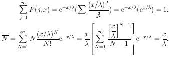
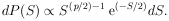
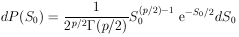
13. POISSON DISTRIBUTION
A common type of problem which falls into this category
is the determination of a cross section or a mean free path.
For a mean free path , the
probability of getting an event
in an interval dx is
dx / . Let
P(0, x) be the probability of
getting no events in a length x. Then we have
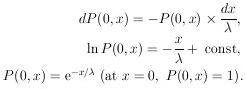
| (19)
|
Let P(N, x) be the probability of finding N
events in a
length x. An element of this probability is the joint probability
of N events at
dx1, ..., dxN times the probability
of no events in the remaining length:
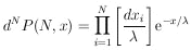
| (20)
|
The entire probability is obtained by integrating over the
N-dimensional space. Note that the integral
does the job except that the particular probability element in
Eq. (20) is swept through N! times. Dividing by N! gives
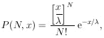
| the Poisson
distribution
| (21)
|
As a check, note
Likewise it can be shown that
 =
=  .
Equation (21) is often expressed in terms of
:
.
Equation (21) is often expressed in terms of
:
| the Poisson
distribution
| (22)
|
This form is useful in analyzing counting experiments. Then
the "true" counting rate is
.
We now consider the case in which, in a certain experiment,
N events were observed. The problem is to determine the
maximum-likelihood solution for
and its
error:
Thus we have
and by Eq. (7),
In a cross-section determination, we have
=
 x
,
where is
the number of target nuclei per cm3 and x is the total
path length. Then
x
,
where is
the number of target nuclei per cm3 and x is the total
path length. Then
In conclusion we note that
:
14. GENERALIZED MAXIMUM-LIKELIHOOD METHOD
So far we have always worked with the standard maximum-likelihood
formalism, whereby the distribution functions are
always normalized to unity. Fermi has pointed out that the
normalization requirement is not necessary so long as the basic
principle is observed: namely, that if one correctly writes
down the probability of getting his experimental result, then
this likelihood function gives the relative probabilities of
the parameters in question. The only requirement is that the
probability of getting a particular result be correctly written.
We shall now consider the general case in which the probability
of getting an event in dx is F(x)dx, and
is the average number of events one would get if the same
experiment were repeated many times. According to Eq. (19),
the probability of getting no events in a small finite interval
x is
The probability of getting no events in the entire interval
xmin < x < xmax is the
product of such exponentials or
The element of probability for a particular experimental result
of N events at
x = x1, ... , xN is then
Thus we have
and
The solutions
i =
i* are still
given by the M simultaneous equations:
The errors are still given by
where
The only change is that N no longer appears explicitly in the
formula
A derivation similar to that used for Eq. (8) shows that N is
already taken care of in the integration over F(x).
In a private communication, George Backus has proven,
using direct probability, that the Maximum-Likelihood Theorem
also holds for this generalized maximum-likelihood method and
that in the limit of large N there is no method of estimation
that is more accurate. Also see Sect. 9.8 of
Ref. 6.
In the absence of the generalized maximum-likelihood method
our procedure would have been to normalize
F(; x) to unity by
using
For example, consider the sample containing just two radioactive
species, of lifetimes
1 and
2. Let
3 and
4 be the two
initial decay rates. Then we have
where x is the time. The standard method would then be to use
which is normalized to one. Note that the four original
parameters have been reduced to three by using
5
4 /
3. Then
3 and
4 would be found
by using the auxiliary equation
the total number of counts. In this standard procedure the equation
must always hold. However, in the generalized maximum-likelihood
method these two quantities are not necessarily equal.
Thus the generalized maximum-likelihood method will give a different
solution for the
i, which should,
in principle, be better.
Another example is that the best value for a cross section
is not obtained by the
usual procedure of setting
L = N (the
number of events in a path length L). The fact that one has
additional prior information such as the shape of the angular
distribution enables one to do a somewhat better job of calculating
the cross section.
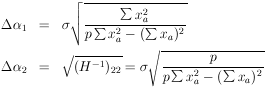
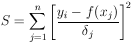
15. THE LEAST-SQUARES METHOD
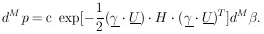
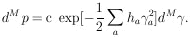
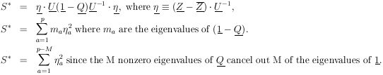
Until now we have been discussing the situation in which
the experimental result is N events giving precise values
x1, ... , xN where the
xi may or may not, as the case may be, be all different.
From now on we shall confine our attention to the case
of p measurements (not p events) at the points
x1, ... , xp. The
experimental results are (y1 ±
1),
... ,(yp ±
p). One such type
of experiment is where each measurement consists of Ni
events.
Then yi = Ni and is
Poisson-distributed with
i =
sqrt[Ni]. In
this case the likelihood function is
and
We use the notation
 (i; x) for the
curve that is to be fitted
to the experimental points. The best-fit curve corresponds to
i =
i*. In this case
of Poisson-distributed points, the
solutions are obtained from the M simultaneous equations
(i; x) for the
curve that is to be fitted
to the experimental points. The best-fit curve corresponds to
i =
i*. In this case
of Poisson-distributed points, the
solutions are obtained from the M simultaneous equations
If all the Ni >> 1, then it is a good
approximation to
assume each yi is Gaussian-distributed with standard
deviation
i. (It is better
to use i rather
than Ni for
i2 where
i can
be obtained by integrating
(x)
over the ith interval.) Then
one can use the famous least squares method.
The remainder of this section is devoted to the case in
which yi are Gaussian-distributed with standard
deviations i.
See Fig. 4. We shall now see that the
least-squares method is
mathematically equivalent to the maximum likelihood method. In
this Gaussian case the likelihood function is
| (23)
|
where
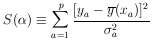
| (24)
|
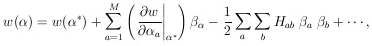
|
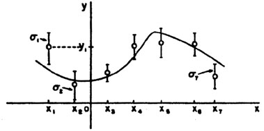
Figure 4.
(x) is
a function of known shape to be fitted to the 7 experimental points.
|
The solutions
i =
i* are given by
minimizing
S() (maximizing
w):

| (25)
|
This minimum value of S is called S*, the least squares sum.
The values of i
which minimize are called the least-squares
solutions. Thus the maximum-likelihood and least-squares solutions
are identical. According to Eq. (11), the least-squares
errors are
Let us consider the special case in which
(i; x) is
linear in the i:
(Do not confuse this f (x) with the f (x) on
page 2.)
Then
| (26)
|
Differentiating with respect to
j gives
| (27)
|
Define
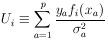
| (28)
|
Then
In matrix notation the M simultaneous equations giving the
least-squares solution are
| (29)
|
is the solution for the
*'s. The errors in
are
obtained using Eq. 11. To summarize:
| (30)
|
Equation (30) is the complete procedure for calculating the
least squares solutions and their errors. Note that even though
this procedure is called curve-fitting it is never necessary
to plot any curves. Quite often the complete experiment may
be a combination of several experiments in which several different
curves (all functions of the
i) may be jointly
fitted. Then the S-value is the sum over all the points on all the
curves. Note that since
w(*) decreases by
½ unit when one
of the j has the
value (i* ±
j),
the S-value must increase by one unit. That is,
Example 5 Linear regression with equal errors
(x) is
known to be of the form
(x) =
1 +
2x. There
are p experimental measurements
(yj ±
).Using Eq. (30) we have
These are the linear regression formulas which are programmed
into many pocket calculators. They should not be used in
those cases where the
i are not all the
same. If the i
are all equal, the errors
or
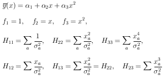
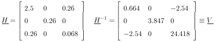
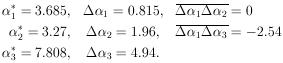
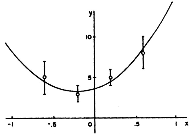
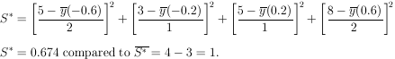
Example 6 Quadratic regression with unequal errors
The curve to be fitted is known to be a parabola. There
are four experimental points at
x = - 0.6, - 0.2, 0.2, and 0.6.
The experimental results are
5 ± 2, 3 ± 1, 5 ± 1, and 8 ± 2. Find the best-fit curve.
(x) =
(3.685 ± 0.815) + (3.27 ± 1.96)x + (7.808 ±
4.94)x2 is the
best fit curve. This is shown with the experimental points
in Fig. 5.
|
Figure 5. This parabola is the least
squares fit to the 4 experimental points in Example 6.
|
Example 7
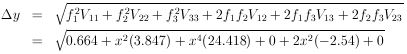
In example 6 what is the best estimate of y at x = 1? What
is the error of this estimate?
Solution: Putting x = 1 into the above equation gives
y is obtained using
Eq. 12.
Setting x = 1 gives
So at x = 1, y = 14.763 ± 5.137.
Least Squares When the yi are Not Independent
Let
be the error matrix-of the y measurements. Now we shall treat
the more general case where the off diagonal elements need not
be zero; i.e., the quantities yi are not
independent. We see
immediately from Eq. 11a that the log likelihood function is
The maximum likelihood solution is found by minimizing
where
| Generalized least squares sum
|
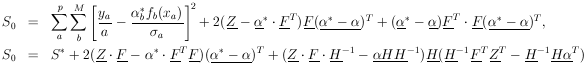
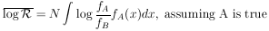
16. GOODNESS OF FIT, THE
2DISTRIBUTION
The numerical value of the likelihood function at
(*) can, in principle, be used as
a check on whether one is using the correct type of function for
f (; x). If one is
using the wrong f, the likelihood function will be lower in
height and of greater width. In principle, one can calculate,
using direct probability, the distribution of
(*) assuming a particular true
f (0,
x). Then the probability of getting an
(*) smaller than the value
observed would be a useful
indication of whether the wrong type of function for f had been
used. If for a particular experiment one got the answer that
there was one chance in 104 of getting such a low value of
(*), one would seriously question
either the experiment or the function
f (;x) that
was used.
In practice, the determination of the distribution of
(*) is usually an impossibly
difficult numerical integration
in N-dimensional space. However, in the special case of the
least-square problem, the integration limits turn out to be
the radius vector in p-dimensional space. In this case we use
the distribution of
S(*) rather than of
(*). We shall first consider the
distribution of
S(0).
According to Eqs. (23) and (24) the probability element is
Note that S =
2,
where is the
magnitude of the radius vector
in p-dimensional space. The volume of a p-dimensional sphere
is U  p. The
volume element in this space is then
p. The
volume element in this space is then
Thus
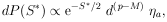
The normalization is obtained by integrating from S = 0 to
S = .
| (30a)
|
where
S
S(0).
This distribution is the well-known
2 distribution with
p
degrees of freedom. 2
tables of
for several degrees of freedom are commonly available - see
Appendix V for plots of the above integral.
From the definition of S (Eq. (24)) it is obvious that
 0 = p. One
can show, using Eq. (29) that
0 = p. One
can show, using Eq. (29) that
 = 2p. Hence,
one should be suspicious if his experimental result gives an
S-value much greater than
= 2p. Hence,
one should be suspicious if his experimental result gives an
S-value much greater than
Usually is not known. In
such a case one is interested in the distribution of
Fortunately, this distribution is also quite simple. It is
merely the 2
distribution of (p - M) degrees of freedom, where
p is the number of experimental points, and M is the number
of parameters solved for. Thus we haved
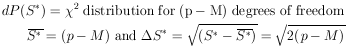
| (31)
|
Since the derivation of Eq. (31) is somewhat lengthy, it is
given in Appendix II.
Example 8
Determine the 2
probability of the solution to Example 6.
According to the 2
table for one degree of freedom the probability of getting
S* > 0.674 is 0.41. Thus the experimental data
are quite consistent with the assumed theoretical shape of
Example 9 Combining Experiments
Two different laboratories have measured the lifetime of
the K10 to be
(1.00 ± 0.01) × 10-10 sec and
(1.04 ± 0.02) × 1010 sec
respectively. Are these results really inconsistent?
According to Eq. (6) the weighted mean is
* = 1.008 ×
10-10 sec.
(This is also the least squares solution for
KO.
Thus
According to the 2
table for one degree of freedom, the probability of getting
S* > 3.2 is 0.074. Therefore, according
to statistics, two measurements of the same quantity should be
at least this far apart 7.4% of the time.
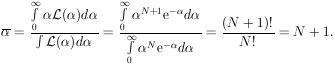
APPENDIX I: PREDICTION OF LIKELIHOOD RATIOS
An important job for a physicist who plans new experiments
is to estimate beforehand just how many events will be
needed to "prove" a certain hypothesis. The usual procedure
is to calculate the average logarithm of the likelihood ratio.
The average logarithm is better behaved mathematically than
the average of the ratio itself. We have
| (32)
|
or
Consider the example (given in Section 3) of
the K+ meson. We
believe spin zero is true, and we wish to establish betting odds
of 104 to 1 against spin 1. How many events will be needed for
this? In this case Eq. (32) gives
Thus about 30 events would be needed on the average. However,
if one is lucky, one might not need so many events. Consider
the extreme case of just one event with
x = 0 :  would then
be infinite and this one single event would be complete proof
in itself that the K+ is spin zero. The fluctuation (rms
spread) of log for a
given N is
would then
be infinite and this one single event would be complete proof
in itself that the K+ is spin zero. The fluctuation (rms
spread) of log for a
given N is
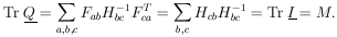
APPENDIX II: DISTRIBUTION OF THE LEAST-SQUARES SUM
We shall define the vector
Zi
yi /
i and the matrix
Fij
fj(xi) /
i.
Note that
H = FT
. F by Eq. (27),

| (33)
|
Then
| (34)
|
where the unstarred is used
for 0.
using Eq. (34). The second term on the right is zero because of
Eq. (33).
| (34)
|
Note that
If qi is an eigenvalue of
Q, it must be equal qi2,
an eigenvalue of Q2. Thus qi
= 0 or 1. The trace of Q is
Since the trace of a matrix is invariant under a unitary
transformation, the trace always equals the sum of the eigenvalues
of the matrix. Therefore M of the eigenvalues of Q are one,
and (p - M) are zero. Let U be the unitary matrix
which diagonalizes Q (and also
(1 - Q)). According to Eq. (35),
Thus
where S* is the square of the radius vector in (p -
M)-dimensional
space. By definition (see Section 16) this is the
2
distribution with (p - M) degrees of freedom.
APPENDIX III. LEAST SQUARES WITH ERRORS IN BOTH VARIABLES
Experiments in physics designed to determine parameters
in the functional relationship between quantities x and y
involve a series of measurements of x and the corresponding y.
In many cases not only are there measurement errors
 yi for
each yj, but also measurement errors
xj for
each xj. Most
physicists treat the problem as if all the
xj = 0
using the
standard least squares method. Such a procedure loses accuracy
in the determination of the unknown parameters contained in
the function y = f (x) and it gives estimates of
errors which are smaller than the true errors.
yi for
each yj, but also measurement errors
xj for
each xj. Most
physicists treat the problem as if all the
xj = 0
using the
standard least squares method. Such a procedure loses accuracy
in the determination of the unknown parameters contained in
the function y = f (x) and it gives estimates of
errors which are smaller than the true errors.
The standard least squares method of Section 15 should be
used only when all the
xj <<
yi.
Otherwise one must replace the weighting factors
1 / i2
in Eq. (24) with
(j)-2
where
| (36)
|
Eq. (24) then becomes
| (37)
|
A proof is given in Ref. 7.
We see that the standard least squares computer programs may
still be used. In the case where
y = 1 +
2x one may use
what
are called linear regression programs, and where y is a polynomial
in x one may use multiple polynomial regression programs.
The usual procedure is to guess starting values for
ðf / ð x and then solve for the parameters
j* using Eq. (30)
with
j replaced by
j. Then new
[ðf / ð x]j can
be evaluated and the procedure repeated.
Usually only two iterations are necessary. The effective
variance method is exact in the limit that
ðf / ð x is constant over the region
xj. This
means it is always exact for linear regressions.


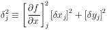
APPENDIX IV. NUMERICAL METHODS FOR MAXIMUM LIKELIHOOD AND
LEAST SQUARES SOLUTIONS
In many cases the likelihood function is not analytical
or else, if analytical, the procedure for finding the
j* and
the errors is too cumbersome and time consuming compared to
numerical methods using modern computers.
For reasons of clarity we shall first discuss an
inefficient, cumbersome method called the grid method. After
such an introduction we shall be equipped to go on to a more
efficient and practical method called the method of steepest descent.
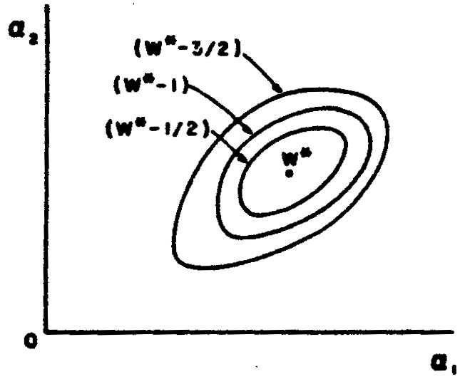
The grid method
If there are M parameters
1, ... ,
M to be
determined one
could in principle map out a fine grid in M-dimensional space
evaluating w() (or
S()) at each
point. The maximum value
obtained for w is the maximum likelihood solution w*. One
could then map out contour surfaces of
w = (w* - ½), (w* - 1), etc. This
is illustrated for M = 2 in Fig. 6.

|
Figure 6. Contours of fixed w
enclosing the max. likelihood solution w*.
|
In the case of good statistics the contours would be small
ellipsoids. Fig. 7 illustrates a case of poor
statistics.

|
Figure 7. A poor statistics case of Fig. 6.
|
Here it is better to present the (w* - ½) contour
surface (or the
(S* + 1) surface) than to try to quote errors on
. If
one is to quote errors it should be in the form
1-
< 1 <
1+
where
1- and
1+ are
the extreme excursions the surface makes
in 1 (see
Fig. 7). It could be a serious mistake to quote
a- or a+ as the errors in
1.
In the case of good statistics the second derivatives
ð2w /
ða
ðb = -
Hab could be found numerically in the region near
w*. The errors in the
's are then found by
inverting the H-matrix to obtain the error matrix for
; i.e.,
= (H-1)ij. The second derivatives can be found
numerically by using
In the case of least squares use
Hij = ½ ðS /
ði
ðj .
So far we have for the sake of simplicity talked in terms
of evaluating w()
over a fine grid in M-dimensional space.
In most cases this would be much too time consuming. A rather
extensive methodology has been developed for finding maxima or
minima numerically. In this appendix we shall outline just one
such approach called the method of steepest descent. We shall
show how to find the least squares minimum of
S(). (This is
the same as finding a maximum in
w()).
Method of Steepest Descent
At first thought one might be tempted to vary
1 (keeping
the other 's fixed) until a
minimum is found. Then vary
2
(keeping the others fixed) until a mew minimum is found, and
so on. This is illustrated in Fig. 8 where
M = 2 and the errors
are strongly correlated. But in Fig. 8 many
trials are needed.
This stepwise procedure does converge, but in the case of
Fig. 8, much too slowly. In the method of
steepest descent one moves against the gradient in
-space:
So we change all the 's
simultaneously in the ratio ðS /
ð1 :
ðS /
ð2 :
ðS /
ð3 : ...
. In order to find the minimum along
this line in -space one
should use an efficient step size.
An effective method is to assume S(s) varies quadratically
from the minimum position s* where s is the distance along
this line. Then the step size to the minimum is
where S1, S2, and
S3 are equally spaced evaluations of
S(s) along s with step size
s starting from
s1; i.e., s2 = s1
+ s,
s3 = s1 +
2s. One or two
iterations using the above formula will
reach the minimum along s shown as point (2) in
Fig. 9. The
next repetition of the above procedure takes us to point (3) in
Fig. 9. It is clear by comparing
Fig. 9 with Fig. 8 that the
method of steepest descent requires much fewer computer evaluations
of S() than does the
one variable at a time method.

|
Figure 9. Same as
Fig. 8, but using the
method of steepest descent.
|
Least Squares with Constraints
In some problems the possible values of the
j are restricted
by subsidiary constraint relations. For example, consider
an elastic scattering event in a bubble chamber where the
measurements yj are track coordinates and the
i are track
directions and momenta. However, the combinations of
i that are
physically possible are restricted by energy-momentum conservation.
The most common way of handling this situation is to use the 4
constraint equations to eliminate 4 of the
's in
S(). Then S is
minimized with respect to the remaining
's. In this example
there would be (9 - 4) = 5 independent
's: two for orientation
of the scattering plane, one for direction of incoming track in
this plane, one for momentum of incoming track, and one for
scattering angle. There could also be constraint relations among
the measurable quantities yi. In either case, if the
method of
substitution is too cumbersome, one can use the method of Lagrange
multipliers.
In some cases the constraining relations are inequalities rather
than equations. For example, suppose it is known that
1 must be
a positive quantity. Then one could define a new set of
's where
(1')2 =
1,
2' =
2, etc. Now if
S(') is minimized no
non-physical values of a will be used in the search for the minimum.
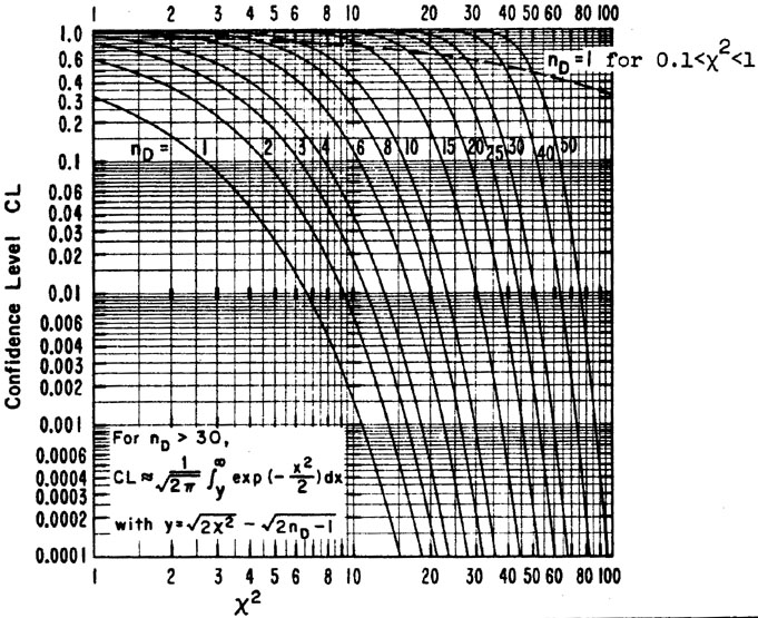
Appendix V. Cumulative Gaussian and Chi-Squared
Distributions
The 2 confidence
limit is the probability of Chi-squared exceeding the observed value; i.e.,
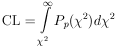
where Pp for p degrees of freedom is given by
Eq. (30a).
Gaussian Confidence Limits
Let 2 =
[x / ]2.
Then for nD = 1,
Thus CL for nD is twice the area under a single
Gaussian tail. For example the nD = 1 curve for
2 = 4 has a value of
CL = 0.046.
This means that the probability of getting
| x|  2 is 4.6% for
a Gaussian distribution.
2 is 4.6% for
a Gaussian distribution.
REFERENCES
Frank Solmitz, Ann. Rev. Nucl. Sci. 14, 375 (1964)
In 1958 it was common to use probable error rather than
standard deviation. Also some physicists would deliberately
multiply their estimated standard deviations by a
"safety" factor (such as ). Such
practices are confusing
to other physicists who in the course of their work must
combine, compare, interpret, or manipulate experimental
results. By 1980 most of these misleading practices had
been discontinued.
An equivalent statement is that in the inverse probability
approach (also called Baysean approach) one is implicitly
assuming that the prior probabilities are equal.
H. Cramer, Mathematical Methods of Statistics,
Princeton University Press, 1946.
M. Annis, W. Cheston, and H. Primakoff, Rev. Mod. Phys.
25, 818 (1953).
A. G. Frodesen, O. Skjeggestad, and H. Tofte,
Probability
and Statistics in Particle Physics. (Columbia University
Press, 1979) ISBN 82-00-01906-3. The title is misleading,
this is an excellent book for physicists in all fields
who wish to pursue the subject more deeply than is done
in these notes.
J. Orear, "Least Squares When Both Variables have
Uncertainties", Amer. Jour. Phys., Oct. 1982.
Some statistics books written specifically for physicists
are:
H. D. Young, "Statistical Treatment of Experimental Data,"
(McGraw-Hill Book Co., New York, 1962).
P. R. Bevington, "Data Reduction and Error Analysis for
the Physical Sciences," (McGraw-Hill Book Co., New York
1969).
W. T. Eadie, D. Drijard, F. E. James, M. Roos, and
B. Sadoulet, "Statistical Methods in Experimental
Physics," (North-Holland Publishing Co., Amsterdam-London,
1971).
S. Brandt, "Statistical and Computational Methods in
Data Analysis," second edition (Elsevier North-Holland
Inc., New York, 1976.)
S. L. Meyer, "Data Analysis for Scientists and Engineers"
(John Wiley and Sons, New York, 1975).
Reprinted from Rev. Mod. Phys. 52, No. 2, Part 11, April
1980 (page 536).